|
|
 |
||||||||||||||||||||||||||||||||||||||||||||||||||||||||||||||||||||||||||
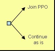
Decision TreesIntroduction to Decision Trees Read► This section introduces decision trees, a tool for choosing between alternatives. We have already introduced tools for measuring a decision maker’s utility and uncertainty. These tools are useful for many problems, but their usefulness is limited when a series of intervening events is likely. When a sequence of events must be analyzed, decision trees provide a means to consider both utility and uncertainty. Utility Modeling► Measuring Uncertainty► The first part of this section defines decision trees, shows how they are constructed, and describes how they can be analyzed using mathematical expectations. The second part introduces "folding back," a concept useful for analysis of decision trees. The Benefit Manager’s DilemmaThroughout this section, we will return to the dilemma faced by the benefits manager of a corporation with 992 employees, all of them covered by an indemnity health insurance program. Employees can seek care from any physician and, after satisfying an annual deductible, must pay only a co-payment, with the employer paying the remainder. A preferred provider organization (PPO) has approached the benefits manager and offered to discount services to employees who use its clinic and hospital. As an inducement, the PPO wants the company to increase the deductible and/or co-payment required of employees who use other providers. Employees would still be free to seek care from any provider, but it would cost them more. The logic of the arrangement is simple—the PPO can offer a discount because it expects a high volume of sales. Nevertheless, the benefits manager wonders what would happen if employees start using the preferred provider. In particular, an increase in the rate of referrals and clinic visits could easily eat away the savings on the price per visit. Change of physicians could also alter the employees’ place of and rate of hospitalization, which would likewise threaten the potential savings. We should clarify some terminology before proceedings. Discount refers to proposed charges at the PPO compared to what the employer would pay under its existing arrangement with the current provider. Deductible is a minimum sum that must be exceeded before the health plan begins to pick up the bill. Co-payment is the portion of the bill the employee must pay after the deductible is exceeded. Describing the ProblemIn a tree, the sequence of events tells the central line of the story. If the analysis measures uncertainty about cost of care while ignoring these intervening events, then the sequence of the events and certain important relationships are lost. It would be like reading the beginning and ending of a novel: it may be effective at getting the message across but not at communicating the story. Imagine a tree with a root, a trunk, and many branches. Lay it on its side, and you have an image of a decision tree. The word tree has a special meaning in graph theory. No branch of the tree is ever connected to the root, trunk, or branch leading to it. Thus, a tree is not circular; you cannot begin at one place, travel along the tree, and return to the same place. Because a decision tree shows the temporal sequence—events to the left happen before events to the right—we begin describing a decision tree with its trunk. The root of the tree, placed to the left and shown as a small square, represents a decision. There are at least two lines emanating from this decision node. Each line corresponds to one option. In our example, two lines represent the options of signing a contract with the preferred provider or continuing with the status quo (See Figure 1).
Figure 1: An
Example Decision Node |
||||||||||||||||||||||||||||||||||||||||||||||||||||||||||||||||||||||||||
|
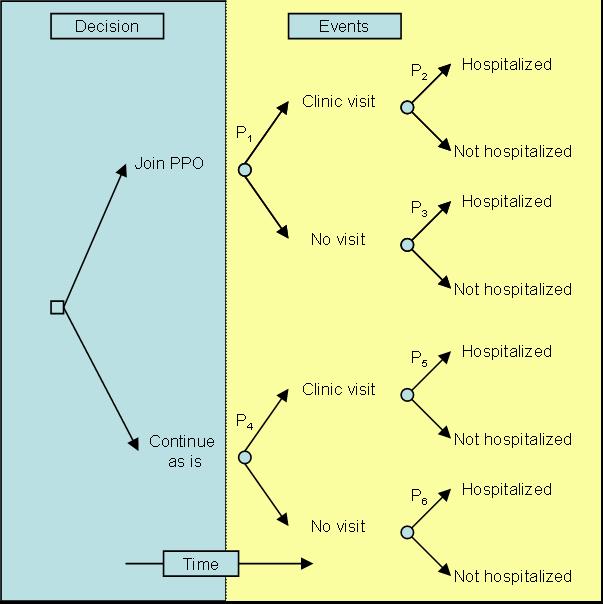
The second component of a decision tree is a chance node. This node shows the occurrence of events over which the decision maker has no direct control. From a chance node several lines are drawn, each showing a different possible event. Suppose that joining a PPO will change the utilization of hospital and outpatient care. Figure 2 shows a portrayal of these events. Note that the chance node is identified by a circle. The distinction between circles and boxes indicates whether the decision maker has control over the events that follow a node. Figure 2 suggests that, for people who join the preferred provider, there is an unspecified probability of hospitalization, outpatient care, or no utilization. We mark these probabilities P1, P2 ,... , P6 (It is the practice to place probabilities above the lines leading to the events they are concerned with.)
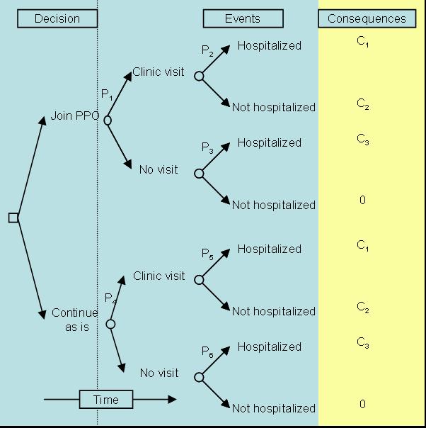
Figure 2: Possible events are placed to the right of the decision The third element in a decision tree is the consequences. While the middle of the tree shows events following the decision, the right side, at the end of the branches, shows the consequences of these events. Suppose, for the sake of simplicity, that the benefits manager is only interested in costs, and not just costs to anybody but costs to the employer, which exclude co-payments and deductibles paid by the employee. Since we do not yet know these costs, we label hospital and clinic charges C1, C2, . . . , C4 and show them at the right. Figure 3 represents the three major elements of a decision tree: decisions, chance events, and consequences (in this case, costs). In addition to these elements, a tree contains a temporal sequence— events at the left precede events on the right.
Figure 3: Consequences (values, costs, or utilities) are placed to the right of the tree Solicitation ProcessA decision tree, once analyzed and reported, indicates a preferred option and the rationale for choosing it. Such a report communicates the nature of the decision to other members of the organization. The tree and the final report on the preferred option are important organizational documents that can influence people, for better or worse, long after the original decision makers have left. While the analysis and the final report are important by themselves, the process of gathering data and modifying the tree are equally important—perhaps more so. The process helps in several ways:
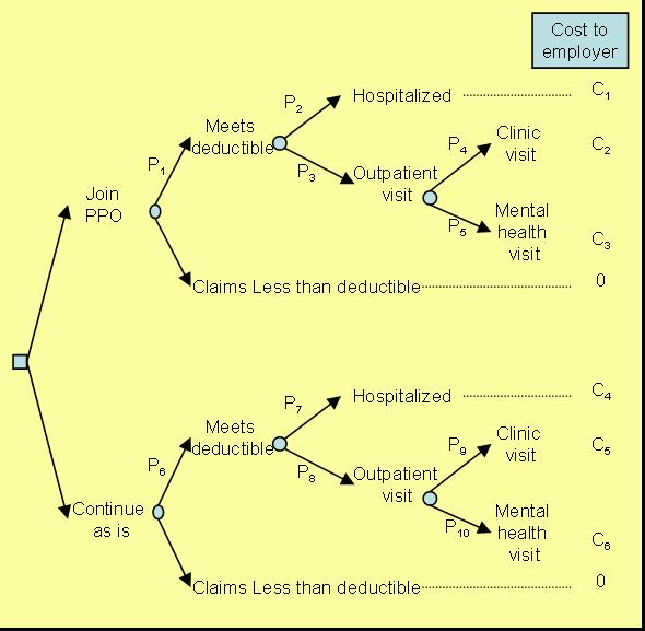
Once a basic tree structure has been organized, it is important to return to the decision makers and see if all relevant issues have been modeled. When we showed Figure 3 to the decision makers, they pointed out the following additional changes:
We revised the model to reflect these issues, and in subsequent meetings the client added still more details, particularly about the relationship among the co-payment, discount, and deductible. This is important because the order in which these terms are incorporated changes the value of the different options. Negotiations between the employer and the preferred provider have suggested that the discount is on the first dollar, before the employee pays the co-payment. Employees had a $200 individual and a $500 family deductible for costs paid for clinics or hospitalization. The insurance plan required meeting the deductible before the co-payment. Once these considerations were incorporated, we reached the revised model presented in Figure 4.
Figure 4: Revised Tree In summary, development of the decision tree proceeds toward increased specification and complexity. The early model is simple, later models are more sophisticated, and the final one may be too complicated to show all elements graphically, and is used primarily for analytical purposes. Each step toward increasing specification involves interaction with the decision maker – an essential element to a successful analysis. Estimating the ProbabilitiesIn a decision tree, each probability is conditioned on events preceding it. Thus P1 in Figure 4 is not the probability of hospitalization but the probability of hospitalization given the person has met the deductible and has joined the PPO. It is important not to confuse conditional probabilities with marginal probabilities. Conditional probabilities for the decision tree can be estimated by either analyzing objective data or obtaining subjective opinion of the experts (see chapter on Measuring uncertainty). The probabilities needed for the lower part of the tree, P6 through P10 can be assessed by reviewing the employers current experiences. We reviewed one year of the data from the employer's records and estimated the various probabilities needed for the lower part of the tree. The probabilities for the upper part of the tree are more difficult to assess as they require a speculation regarding what might happen if employees utilize the preferred clinic. The decision maker identified several factors that might affect what might occur:
To estimate the potential impact of these issues on the probability of hospitalization, we reviewed the literature and brought together a panel of experts familiar with practice patterns of different clinics. We asked them to assess the difference between the PPO and the average clinic in town. We then used the estimates available through the literature to assess the potential impact of these practice differences on utilization rates. Table 1 provides a summary of our synthetic estimate of what might happen to hospitalization rates by joining the PPO. Table 1: Increase in Hospitalization Rates Projected at the Preferred Clinic
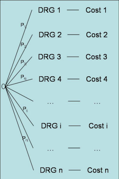
This estimate shows how we gauge the impact of joining the preferred provider by combining the expert’s assessments with the research literature. Although these estimates are at best guesses, they are usually sufficient. Keep in mind that the purpose of these estimates is not to answer precisely to the fourth digit what will happen but whether roughly one option is better than the other. The assumptions made in the analysis can be tested by conducting "sensitivity analysis," a process in which one or two estimates are changed slightly to see if it would lead to entirely different decisions. In our example, the analysis was not sensitive to small changes in probabilities but was sensitive -- as it will become clear shortly -- to the cost per hospitalization. Figure 5 provides a summary of estimated probabilities for both the upper and lower part of the tree. Estimating Hospitalization CostsIn estimating cost per hospitalization, we assume that the employees will incur the same charges as current patients at the preferred hospital. However, this is misleading because the provider, as a large referral center, treats patients who are extremely ill. Company employees are unlikely to be as sick, and thus will not incur equally high charges, so we adjust charges to reflect this difference. We make this adjustment using a system developed by Medicare to measure differences in case mix of different institutions. In this system, each group of diseases is assigned a cost relative to the average case. Patients with diseases requiring more resources have higher costs and are assigned values greater than one. Similarly, patients with relatively inexpensive diseases receive a value less than one. As Figure 5 shows, each health care organization is assumed to different diseases.
Figure 5: A Decision Tree Structure for Calculating Case
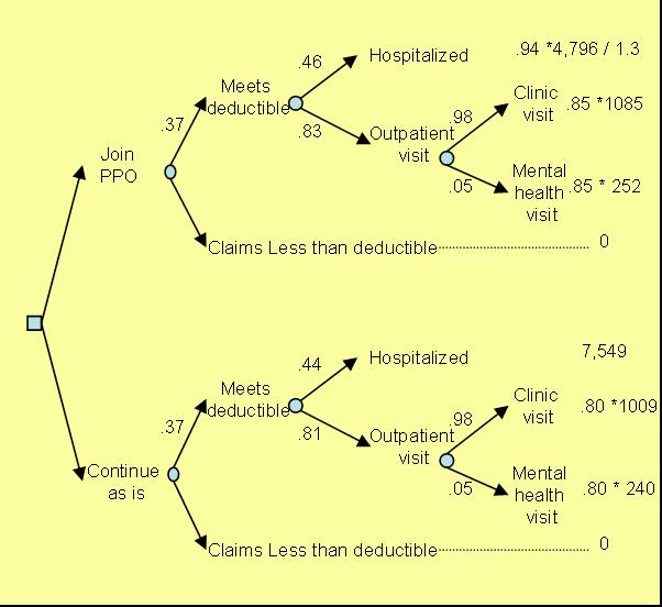
Mix at Hospital "J" The case mix for an institution is the cost of the Diagnostic Related Group (DRG) weighted by the frequency of occurrence of the DRG at that institution. Suppose Medicare has set the cost of ith DRG to be Ci, and Pij measures the frequency of occurrence of DRG i at hospital j, then: Case mix for hospital j = ∑Ci Pij For i =1, ..., n The ratio of two case mix calculations at two different institutions is called a case mix factor. It shows how the two institutions are different. A case mix factor of 1 suggest that the two institutions have patients of similar diseases. Tertiary hospitals tend to have a case mix factor that is above one when compared to community hospitals, indicating that they see sicker patients. To measure the cost that bank employees would have at the PPO hospital, we reviewed employee records at the bank and patient records at the preferred hospital. We constructed a case mix index for each. Employees had a case mix of 0.90, suggesting that these employees were not as sick as the average Medicare employees; the case-mix index at the preferred hospital that year was 1.17, suggesting that patients at the PPO hospital were sicker than the average Medicare patient. We calculated the ratio of the two as 1.3. This suggested that the diseases treated at the preferred hospital were about 30 percent more costly than those typically faced by employees, so we proportionally adjusted the average hospitalization charges at the PPO. The average hospitalization cost at the PPO was $4,796. Using the case mix difference, we predicted that if bank employees were hospitalized at the PPO hospital, they would have an average of $4,796/1.3, or roughly 30% less cost. Figure 6 shows the estimated costs for the lower and upper parts of the tree. Costs reported in the Figure reflect cost per employee's family per year.
Figure 6: Decision Tree with Estimated Costs and
Probabilities Analysis of TreesThe analysis of decision trees is based on the concept of expectation. In everyday use, the word suggests some sort of anticipation about the future rather than an exact formula. In this everyday sense, one may ask, “What do you expect a preferred provider to cost our company?” and you are free to answer as your assumptions and intuitions suggest. In mathematics, expectation is precisely defined. I f you believe that costs c1, c2, .. . , Cn may happen with probabilities P1, P2, ... , Pn then the mathematical expectation is: Expected cost = ∑Pi * ci For i =1, ..., n Each node of a tree can be replaced by its expected cost. The expected cost at a node is the sum of costs weighted by the probability of their occurrence. Consider for example the node for employees who under current situation meet their deductible and have outpatient visits. They have 98% chance of having an outpatient visit costing $1,009 per year per person (80% of which is charged to the employer and the rest is paid by the employee). They also have 5% chance of having a mental health visit costing $240 (80% of which is charged to the the employer and the rest to the employee). The expected cost to the employer for outpatient visits per employee per year is then calculated as:
Employer's expected cost for
outpatient visits = 0.98 * 0.80 * 1009 + 0.05 * 0.80 * 240 = 816.8
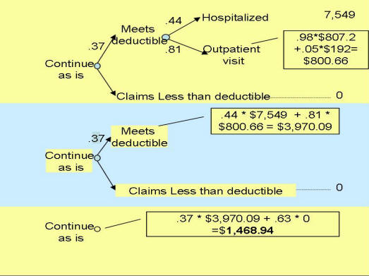
This expected cost can replace the node for outpatient visits in the "Continue as is" situation in the tree. Likewise the process can now be repeated to fold back the tree further and replace each node with its expected cost (see Figure 7 calculating the expected cost of continuing as is through three steps).
Figure 7: Starting from right, each node is replaced with its expected value The employer's expected cost for joining the PPO was calculated to be $871.08 per employee family per year. This is $597.86 per employee's family per year less than the current situation. Since the firm had 992 employees, the analysis suggests almost half million dollars cost saving per year by switching to the PPO. The problem with the folding back method is that it is not easy to represent the calculation in formulas inside programs such as Excel. Too much of the information is visual. There is another way of folding a decision tree that takes advantage of the tree structure and does not require folding back procedures. First, all the probabilities for each path in the tree are multiplied together to find the joint probability of the sequence. For example, after joining the HMO, the joint probability of meeting the deductible and being hospitalized is provided by multiplying o.37 (probability of meeting the deductible for people who join the PPO) by 0.46 (the probability of being hospitalized if you have joined the PPO and met the deductible). To calculate the expected cost/value the joint probability of each path is multiplied by the corresponding cost/value and summed for each option. The following table shows each of the paths in the upper part of the tree in Figure 7, the corresponding joint probability of the sequence and its associated costs:
This information can be used to calculate expected cost by multiplying the cost and the probability of each path and summing the results. Using the terms introduced in Figure 4, the expected cost of joining the PPO can be calculated using the following formula: Expected cost (Joining PPO): P1P2C1 + P1P3P4C2 + P1P3P5C3 Note that the above formula does not show situations that lead to zero cost (not meeting the deductible or meeting the deductible but not having any additional health care utilization). If we wanted to show the path leading to zero cost for employees that do not meet the deductible, we would have to the following terms to the above formula: + (1-P1)0 The expected cost of continuing as is can be calculated as: Expected cost (Continuing as is): P6P7C4 + P6P8P9C5 + P1P6P8C10 When we express expected costs as a formula, it is possible to enter the formula into Excel and ask a series of "what if" questions. The analyst can change values of one variable and see the impact of the change on the expected cost calculations. Sensitivity AnalysisSome analysts mistaken stop the analysis after a preferred option has been identified. This is not the point to end the analysis but the start of real give and take, real understanding of what leads to the choice of one option over another. As we have repeatedly mentioned in this book, the purpose of analysis is to provide insight and not to produce numbers. One way to help decision makers better understand the structure of their decision is to analyze the data to see if the conclusions are particularly sensitive to some inputs. This is called sensitivity analysis. It helps in another way too. Many decision makers are skeptical of the numbers used in the analysis and wonder if the conclusion could be different if the estimated numbers were different. Sensitivity analysis is the process of changing the input parameters until the output (the conclusions) are affected. In other words, it is the process of changing the numbers until the analysis falls apart and conclusions are reversed. Sensitivity analysis starts with changing one single estimate at a time until the conclusion is reversed. Two other point estimates are calculated, one for the best possible scenario and the other for the worst possible scenario. For example, under joining the PPO, the probability of hospitalization given the person has met the deductible is an important estimate about which the decision maker may express reservations. To understand the sensitivity of the conclusions to this probability, three estimates are obtained. One for the probability set to maximum (when everyone is hospitalized) and the other to the minimum (when no one is hospitalized). The expected values of the options are calculated under these circumstances and the following table produced:
Changing this conditional probability leads to a change in the expected cost of joining the PPO. To understand whether the conclusion is sensitive to the changes in this conditional probability, analysts typically plot the changes. The X axis will show the changing estimate, in this case the conditional probability of hospitalization for employees who meet the deductible and have joined the PPO. The Y axis shows the value of the decision options, in this case either the expected cost of joining the PPO or the expected cost of continuing as is. A line is drawn for each option. The Figure below shows the resulting sensitivity graph:
Figure 8: Sensitivity of Conclusions to conditional
probability of hospitalization for Note that in Figure 8, for the most part , joining the PPO is preferred to continuing as is. Only at very high probabilities of hospitalization, which the decision maker might consider improbable, the situation is reversed. The decision is reversed at 0.93. We call this the reversal point. If the estimate is near the reversal point, then the analyst would be concerned. If the estimate is far away, the analyst will be less concerned. The distance between the current estimate of 0.37 and the reversal point of 0.92 suggests that small inaccuracies in estimation of the probability will not matter in the final analysis. What will matter? The answer can be found by conducting sensitivity analysis on each of the parameters in the analysis and finding one in which small changes can lead to decision reversals. The analysis calculates the cost of hospitalization for employees from current hospital costs at the PPO. PPO hospitalization costs are reduced by a factor of 1.3 in order to reflect the case mix of the employed population. It assumes that employed population are less severely sick than the general population at the PPO hospital. What if the analysis was wrong in this estimate? The reversal point for the estimate of case mix is at 0.65, at which point the cost of hospitalization for the employees at the PPO would be estimated to be $6,935. This seemed unlikely as it would have claimed that the bank's employees needed to be significantly sicker than the current patients at the PPO hospital, a national referral center. It is important to find the reversal points for each of the estimate in a decision tree. This can be done by solving an equation where the variable of interest is changed so that it produces an expected value equal to the alternative option. It can also be done more easily in Excel using the Goal Seeking tool. The goal seeking tool is asked to find an estimate for the variable of interest that would make the difference between the two options become zero. So far we have talked about changing one estimate and seeing if it leads to a decision reversal. What if two or more estimates were simultaneously changed? How can we find the sensitivity of our decision to changes in multiple estimates. For example, what if we were wrong both about probability of hospitalization and the cost of hospitalization. To assess the sensitivity of conclusion to simultaneous changes in several estimates, we need to use a technique known as Linear Programming. This technique allows the minimization of an objective subject to constraints on several variables. The absolute difference between the expected value of the two options are minimized subject to constraints imposed by the low and high range of the various estimates. For example, we might minimize the difference between expected cost of joining the HMO and continuing as is subject to case mix ranging from 1 to 1.4 and conditional probability of hospitalization ranging from 0.3 to 0.5. Mathematically, this shown as follows:
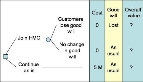
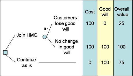
It is difficult to solve linear programs by hand. One possibility is to solve for the worst case scenario. In this situation, we will assume that joining the HMO will lead to the worst rate of hospitalization (0.5) and the worst cost of hospitalization (case mix of 1). Even under this worst case scenario, joining the PPO remains the preferred option. In addition to using the worst case scenarios, it is also possible to use Excel. Excel provides a relatively easy to use Linear Programming tool called Solver. To use this tool you need to use add-in feature under the tool option so that this features is available. Using the Solver, the analyst finds that there are no solutions that would make the difference between "joining the HMO" and "continuing as is" become zero subject to above constraints. Therefore, even with both constraints changing at the same time, there is no reversal of conclusions. Missed PerspectivesThe purpose of any analysis is to provide insight. Often when decision makers review an analysis they can find important issues missed in it. In our example PPO, one decision maker believed that the potential savings were insufficient to counterbalance the political and economic costs of instituting the proposed change. It turned Out that the present health care providers were customers of the client, and that signing a contract with the PPO might alienate them and induce them to take their business elsewhere. Incorporating the risk of losing customers would improve our calculation and help the client decide whether the savings would counterbalance the political costs (more on this in the next section). Furthermore, additional discussion lead to another critical perspective: Would it be better to wait for a better offer from a different provider? We could have reflected the consequences of waiting by placing an additional branch from the decision node, and clearly this would have provided a more comprehensive analysis of the decision. New avenues often open up when an analysis is completed. It is important to remember that one purpose of analysis is to help decision makers understand the components of their problem and to devise increasingly imaginative solutions to it. Therefore, there is no reason to act defensively if a client begins articulating new options and considerations while you present your findings. Instead, encourage the client to discuss the option, and consider modifying the analysis to include it. A serious shortcoming with decision trees is that many clients believe they show every possible option. Actually, there is considerable danger in assuming that the problem is as simple as a tree makes it seem. In our example, many other options may exist for reducing health care costs aside from joining the preferred provider, but perhaps because they were not included in the analysis, they can be ignored by the decision maker, who, like the rest of us, is victim to the “out of sight, out of mind” fallacy (also see Fischhoff et al. 1978). The “myth of analysis” can explain why things not seen are not considered. This is the belief that analysis is impartial and rests on proper assumptions and that a small change will not affect the outcome. Perpetuating this myth prevents further inquiry and imaginative solutions to problems. Decision trees could easily fall into this trap because they appear so comprehensive and logical that decision makers fail to imagine any course of action not explicitly included in them. We can gain more insight into the decision by breaking the final report presentation into two segments. First we summarize the results of the tree and the sensitivity analysis, then we ask the clients to share their ideas about options not modeled in the analysis. If one does not explicitly search for new alternatives, the analysis might do more harm than good. Instead of fostering creativity, it can allow the analyst and decision maker to hide behind a cloak of missed options and poorly comprehended mathematics. Expected Value or UtilitySometimes, consequences of an event are not just additional cost or savings. Sometimes it is important to measure the utility associated with various outcomes. In these circumstances, we measure the value of each consequence in term of its utility and not merely its costs. We then use expected utility instead of the expected cost to fold back the decision tree. When in 1738 Bernoulli was experimenting with the notion of expectation, he noticed that people did not prefer the alternative with highest expected monetary value, that people are not willing to pay a large amount of money for a gamble with infinite expected return. In explanation, Bernoulli suggested that people maximize utility rather than monetary value, and costs should be transformed to utilities before expectations are taken. He named this model expected utility. According to expected utility, if an alternative has n outcomes with costs c1, .. . , Cn, associated probabilities of P1, ... , Pn, and each cost has a particular utility to the decision maker, say u1,. . . , Un then: Expected utility = ∑Pi * ui For i =1, ..., n Bernoulli resolved the paradox of why people would not participate in a gamble with infinite return by arguing that the first dollar gained has a greater utility than the millionth dollar. A beauty of a utility model is that it allows the marginal value of gains and losses to decrease with their magnitude. In contrast, mathematical expectation assigns every dollar the same value. When the costs of outcomes differ considerably, say, when one outcome costs $1,000,000 and another $1,000, we can prevent small gains from being overvalued by using utilities instead of costs. Utilities are also better than costs in testing whether benefits meet the client’s goals. Using costs in the preferred provider analysis, we found that joining the PPO would lead to expected savings of about half a million dollar. Yet, when the client had not acted six months after completing the analysis, it became clear that this saving was not sufficient to cause him to act because non-monetary issues were involved. We could have uncovered this problem if, instead of monetary returns, we had used utility estimates. Earlier, we described how to measure utility over many dimensions, monetary and non-monetary. In the example we have been following, cost was not the sole concern—the firm had many objectives for changing its health care plan. If it wanted only to lower costs, it could have ceased providing health care coverage entirely, or it could have increased the co-payment, The firm was concerned about employees’ reactions, which it anticipated would be based on concerns for quality, accessibility, and, to a lesser extent, cost to employees. If that was the case, a utility model should have been constructed on this basis and the model should have been used to assess the value of each consequence. Utility is also preferable for clients who must consider attitudes toward risk. This is because expected utility, in contrast to expected cost, reflects attitudes toward risk. A risk-neutral individual bets the expected monetary value of a gamble. A risk taker bets more on the same gamble because he or she associates more utility to the high returns. A risk adverse individual cares less for the high returns and bets less. Research shows that most individuals are risk seeking when they can choose between a small loss and a gamble for a large gain and are risk adverse when they must choose between a small gain and a gamble for a large loss (Kahneman and Tversky 1979). A client, especially when trying to decide for an organization, may exclude personal attitudes about risk and request that the analysis of the decision tree be based on expected cost and not expected utility. Thus, the client may prefer to assume a risk-neutral person and behave as if every dollar of gain or loss were equivalent. The advantage of making the risk attitudes explicit is that it leads to insights about one’s own policies; the disadvantage is that such policies may not be relevant to other decision makers. Transformation of costs to values/utilities is important in most situations. But when the analysis is not done for a specific decision maker, monetary values are paramount, the marginal value of a dollar seems constant across the range of consequences, and attitudes toward risk seem irrelevant, then it may be reasonable to explicitly measure the cost and implicitly consider the non-monetary issues. When Alemi and colleagues presented the cost effectiveness of the Preferred provider Organization to the bank executives, the bank did not act on the report. When asked, the executives raised the issue that money was not the sole consideration. Many of the hospital's CEOs were on the bank's executive board. The bank was concerned that by preferring one health care provider, they may lose their goodwill and at extreme the hospital may shift their funds to a competing bank. Figure 9 shows the resulting dilemma faced by the bank:
Figure 9: A Decision Tree Showing Banks Concern Over Losing Healthcare Customers In Figure 9, we show that the bank faces the loss of half a million dollars per year for continuing as is. Alternatively it can join the HMO but faces a chance of losing healthcare customer's goodwill. To further analyze this tree, it is necessary to assess the probability of healthcare organizations losing goodwill and the value or utility associated with the overall impact of both cost and goodwill. If we assume that attitudes towards risk do not matter in this analysis, we could focus on measuring overall value using multi-attribute value model discussed in an earlier chapter. Assume that good will is given a weight of 0.75 and cost saving of half a million dollars per year is given a weight of 0.25. Also assume that the probability of healthcare organizations shifting their funds to other banks is considered to be small, say 1 percent. Figure 10 summarizes the data so far:
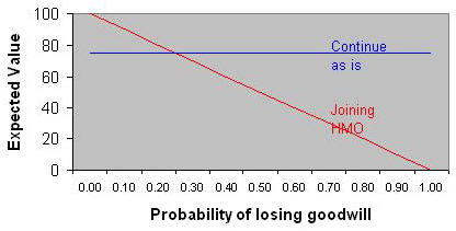
The expected value for joining the HMO can be calculated by folding back starting with the top right hand side. There is a probability of 1% of having an overall value of 25 versus a probability of 99% of having a value of 100. The expected value for this node is 0.01*25+0.99*100 = 99.25. The expected value for "continuing as is" is shown as 75. Therefore, despite the small risk of losing goodwill with some healthcare bank customers, the preferred course of action is to go ahead with the change. We can conduct sensitivity analysis to see at what probability of losing goodwill joining the HMO is no longer reasonable. As the probability of losing goodwill is increased, the value of joining the HMO decreases. At probabilities higher than 0.35, joining the Preferred Provider Organization is no longer preferred over continuing as is.
Sequential DecisionsThere are many situations in which one decision leads to another. A current decision must be made keeping in mind future options. For example, consider a Risk Management department inside a hospital. After a sentinel event in which the patient has been hurt, the Risk Manager can step in with several actions to reduce the probability of a law suit. A patient's bill can be written off. A nurse might be assigned to stay with the patient for the remainder of the hospitalization. Should the risk manager take these steps depends on the effectiveness of the preventive strategy. It also depends on what the hospital will do if sued. For example, if sued the Risk Manager faces the decision to settle out of court or to wait for the verdict. Thus the two decisions are related. The first decision of preventing the law suit is related to the subsequent decision of the disposition of the law suit after it occurs. In this section, we describe how to model and analyze inter-related decisions. As before the most immediate decision is put to the left of a decisions tree followed by its consequences to its right. If there are any related subsequent decisions, it is entered as a node to the right of the decision tree or after specific consequences. For example, the decision to prevent law suits is put to the left in Figure 12. If the law suit occurs, a subsequent decision needs to be made about what to do about the suit. Therefore, following the link that indicates the occurrence of the law suit, a node is entered for how to manage the law suit. To analyze a decision tree with multiple decisions in it, the folding back process is used with one new exception. All nodes are replaced with their expected value/cost as before but the decision node is replaced with the minimum cost or maximum utility/value of the options available at that node. We do so, because obviously at any decision node, the decision maker is expected to maximize his value/utilities or minimize cost.
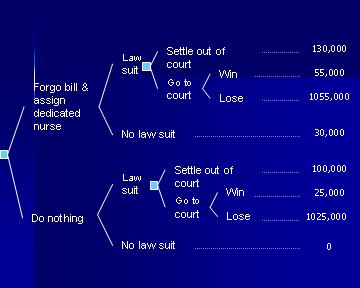
Figure 12: The Decision to Prevent Malpractice Suit In their classic book on Quick Analysis for Busy Decision Makers Behn and Vaupel (1982) suggest how decision tree analysis can be applied to the problem of settling out of court. We apply their suggestions to a potential malpractice situation. As Figure 12 shows, we are estimating the cost of forgoing the hospital bill and assigning a dedicated nurse to the patient at $30,000. If the case is taken to the court, there is $25,000 legal costs. If the hospital loses the case, we are assuming that the verdict will be for one million dollars. Figure 12 summarizes these costs. The question is whether it is reasonable to proceed with the preventive action. To answer this question we need to have three probabilities:
The estimation of these probabilities and the cost payments need to be appropriate to the situation at hand. Figure 12, provides rough estimates for these probabilities and costs but in reality the situation should be tailored to the nature of the patient, the injury and experiences with such law suits. The data in the literature can be used to tailor the analysis to situation at hand. Here are some examples of where the numbers might come from:
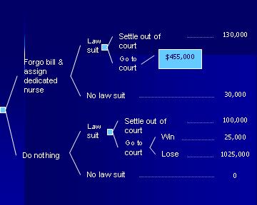
Many similar articles exist in the Medline literature from which both the maximum payout and the probability of these payouts can be assessed. If we assume that the probability of winning in the court for the case at hand is 60% and the probability of law suit is 15% and this probability is reduced to 5% after the preventive action, then we can calculate the optimal decision under these assumptions. To fold back the tree, we start from the top right hand side and first we fold back the node associated with the court outcomes. The expected cost for going to the court is 0.6 * $55,000 + 0.4 * 1055,000 = $455,000. At this point the tree is pruned as in Figure 13.
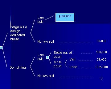
Figure 13: Replacing the court outcomes with their expected costs Settlement out of court will cost 130,000, therefore it is preferred to going to the court. Therefore the expected cost for a law suit is $130,000. Note that in a decision node, we always take the minimum expected cost associated with the options available at this node. This now reduces the tree to Figure 14:
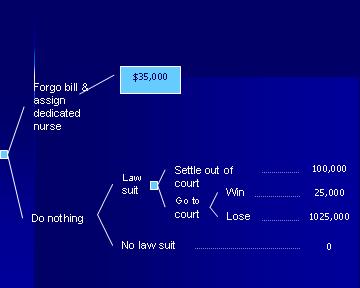
Figure 14: The expected cost for the decision node is the option with minimum cost Next, we can calculate the expected cost for preventive action as 0.05*$130,000+0.95*$30,000 = $35,000. So the final tree looks as Figure 15:
Figure 15: The expected cost of preventing a law suit A similar set of calculations can be carried out for the option of doing nothing. In these circumstances, the expected cost associated with the court case is 0.6 * $25,000 + 0.4 * 1025,000 = $425,000. The preferred option is to settle out of court for $100,000. The expected cost for a law suit is $100,000. The expected cost for doing nothing is 0.15*$100,000 + 0.85 * 0 = $15,000, which is lower than the expected cost of taking preventive action. For this client and this situation (given the probabilities and costs estimated) the best course of action is not to take any preventive action. Sensitivity analysis can help us find the probabilities and costs at which point conclusions are reversed. AssignmentsQuestion A. This problem describes a type of problem typically discussed in Marketing classes, where managers are trained to understand market participation and market share. We have simplified the number of variables and cases in the problem to make it easier to analyze. A typical realistic problem may have hundreds of variables and thousands of cases. Data►
Question B: The following tree shows two events: the first event is the probability of
hospitalization (i.e. the number of persons hospitalized divided by the
number of persons in United States). The second event shows the age given
that the person was hospitalized. This is the conditional probability of
observing a person at a particular age bracket given that the person was
hospitalized. This second event is calculated among hospitalized patients.
The mean cost of hospitalization for persons who were not hospitalized is
zero. the mean cost of hospitalization across two or more age categories is
a weighted average of the cost in the age categories. You can find data to
estimate the various probabilities and costs at a site organized by the
useful site
organized by Agency for Healthcare Quality and Research. Enumerate the tree
and calculate the expected cost of hospitalization for an average person in
United States by folding back the tree to the root node.
Biweekly ProjectAdvanced learners like you, often need different ways of understanding a topic. Reading about decision trees is just one way of understanding this tool. Another way is through creating one. When you do so, you not only learn about decision trees but also gain confidence in your abilities. In the following assignments, you need not collect the probabilities or costs -- you can specify where you might find such information and estimate it as if you had collected it. Option 1: Benchmarking Clinicians
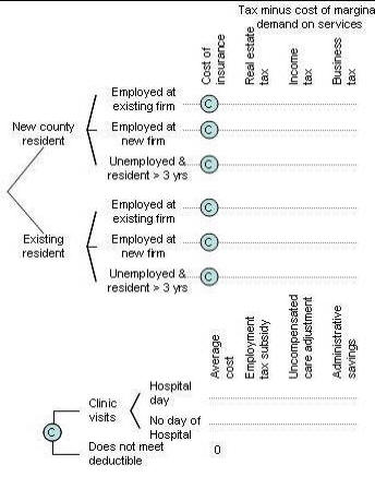
Option 2: Analyzing Proposal to Reform Health Insurance
Note that the decision tree suggests that the premiums for the new plan can be estimated based on current costs and several adjustments. These premiums are then used as input to the portion of tree evaluating impact on taxes. Keep in mind that your tree should reflect the following facts:
Note that it is important to estimate the net taxes raised (i.e. current tax minus the current marginal cost of services) as new migrants will not only pay new taxes but also increase demand for some services. .Please note that the expected cost calculated per resident would need to be multiplied by the number of residents to show the total cost.. Your analysis should include data from the literature or from a knowledgeable expert. Expanding Insurance► Option 3: Analyzing fetal and maternal rights A clinician faced an important dilemma of choosing between fetal and maternal rights. The case was "a 34-year-old female with a 41-week intra-uterine pregnancy. The mother was refusing induction of labor. Without the labor induction, the fetus may die. Despite this risk, the mother desired to pursue a vaginal delivery." What should the clinician do? Model the clinician's decision when the mother refuses to undergo a necessary life saving cesarean for the infant. Make sure that your analysis is based on viability of the infant as well as the intrusiveness of the clinician's intervention. Create a decision tree and solicit the utility of various courses of action under different probabilities. For an example analysis of the same problem see work done by Mohaupt and Sharma PubMed► More
Presentations
To assist you in reviewing the material in this lecture, please see the following resources:
Part one of lecture on introduction to decision tree focuses on elements of a decision tree:
Part two of Introduction to Decision Tree:
Part three of the lecture focuses on folding back a decision tree:
ReferencesBernoulli D. Specimen Theoriae Novae de Mensura Sortis.
Cornmetarri Academiae Scientaiarum Imperialis Petropolitanae V:
175-92, 1738. Also see
Sommer L (translator). Exposition of a New Theory on Measurement of Risk,
Econometrica 22 (1954): 23—26. Bors-Koefoed R, Zylstra S, Resseguie LJ, Ricci BA,
Kelly EE, Mondor MC. Statistical
models of outcome in malpractice lawsuits involving death or neurologically
impaired infants. J
Matern Fetal Med. 1998 May-Jun;7(3):124-31. Behn RD, Vaupel JW.
Quick Analysis for Busy Decision Makers.
Basic Books 1982. Driver JF, Alemi F.
Forecasting without historical data: Bayesian probability models
utilizing expert opinions. J Med Syst. 1995 Aug;19(4):359-74. Fischhoff B, Slovic P, Lichtenstein S. Fault Trees:
Sensitivity of Estimated Failure Probabilities to Problem Presentation.
Journal of Experimental Psychology Human Perception and Performance 4
(2): 330-34, 1978. Rosenblatt RA, Moscovice IS. The Physician as
Gatekeeper: Determinants of Physicians’ Hospitalization Rate.
Medical Care 22 (2): 150-59. 1984. Schoemaker PJH. The Expected Utility Model: Its
Variants, Purposes, Evidence and Limitations.
Center for Decision Research, Graduate School of Business, University
of Chicago, 1982. Also see
Journal of Economic Literature, 1983. Selbst SM, Friedman MJ, Singh SB. Epidemiology and
etiology of malpractice lawsuits involving children in US emergency
departments and urgent care centers. Pediatr Emerg Care. 2005
Mar;21(3):165-9.
Copyright © 1996 Farrokh Alemi, Ph.D. Created on Saturday, September 21, 1996. Most recent revision 04/03/2019. This page is part of the course on Decision Analysis the lecture on Decision Trees. This page is based on a chapter with the same name published by Gustafson DH, Cats-Baril WL, Alemi F. in the book Systems to Support Health Policy Analysis: Theory, Model and Uses, Health Administration Press: Ann Arbor, Michigan, 1992. |
||||||||||||||||||||||||||||||||||||||||||||||||||||||||||||||||||||||||||


 Evaluate
the cost effectiveness of the county self-insuring
Evaluate
the cost effectiveness of the county self-insuring