|
|
 |
|||||||||||||||||||||||||||||||||||||||||||||||||||||||||||||||||||||||||||||||||||||||||||||||||||||||||||||||||||||||||||||||||||||||||||||||||||||||||||||||||||||||||||||||||||||||||||||||||||||||||||||||||||||||||||||||||||||||||||||||||||||||||||||||||||||||||||||||||||||||||||||||||||||||||||||||||||||||||||||||||||||||||||||||||||||||||||||||||||||||||||||||||||||||||||||||||||||||||||||||||||||||||||||
Modeling PreferencesThis chapter introduces a flexible method for modeling decision makers' values and several means of validating such models. We assume that a model is developed jointly by one analyst and one decision maker. If the development process involves a group, the analyst should use the integrative group process discussed in a later chapter. While the model building effort focuses on the interaction between an analyst and a decision maker, it should be obvious that the same process can be used for self-analysis. A decision maker can build a model of his/her own decisions without the help of an analyst. Value models are based on Bernoulli's (1938) recognition that money's value did not always equal its amount. He postulated that increasing amount of income had decreasing value to the wage earner. Value models have received considerable attention from economists and psychologists (Savage .1972; Edwards 1974). A comprehensive and rather mathematical introduction to constructing value models is found in von Winterfeldt and Edwards (1986). This chapter focuses on instructions for making the models and ignores axiomatic/mathematical foundation of multi-attribute value models. Value models quantify a person's preferences. By this, we mean that value models assign numbers to options so that higher numbers reflect more preferred options. These models assume that the decision makers must select from several options and that the selection should depend on grading the preferences for the options. These preferences are quantified by examining the various attributes (characteristics, dimensions, or features) of the options. For example, if decision makers were choosing among different Electronic Medical Record (EMR) systems, the value of the different EMRs could be scored by examining such attributes as “compatibility with legacy systems”, “potential impact on practice patterns” and “cost.” First, the impact of each EMR on each attribute would be scored, this is often called single attribute value function. Second, scores would be weighted by the relative importance of each attribute. Third, the scores for all attributes would be aggregated, often by using a weighted sum. Fourth, the EMR with the highest weighted score would be chosen. If each option was described in terms of n attributes A1, A2, ... , An the option would be assigned a score on each attribute, V(A1), V(A2), ... , V(An). The overall value of an option equals: Value = Function [ V(A1), V(A2), ... , V(An) ] In words, the overall value of an option is a function of the value of the option on each attribute. Why Model Values?Values (attitudes, preferences) play major roles in making management decisions. In organizations, decision making is often very complex and a product of collective action. Frequently, decisions must be made concerning issues on which few data exist, forcing managers to make decisions on the basis of opinions, not fact. Often there is no correct resolution to a problem‑with all options having equally legitimate perspectives and values playing a major role in the final choice. There are many everyday decisions that involve value tradeoffs. Decision such as -- Which software to purchase? Which vendor to contract with? Whether to add a clinic? Whether to add nurses? Whether to shift to float staffing? Whether to buy a piece of equipment? Whether to add a program? Which person to hire? Whether to hire staff or pay overtime? How to balance missions (e.g. providing service with revenue generating activities)? What contractual relationships to enter into? Which quality improvement project to pursue? In all these decisions, the manger has to tradeoff gains in something against other things. Doing a quality improvement project in stroke unit means you do not have resources to do the same in trauma unit. Hiring a technically savvy person may mean you have to put up with socially ineptness. In business, difficult decisions almost always involve trading off various benefits against each other. Most people acknowledge that a manager's decisions involves consideration of value tradeoffs. This is not a revelation. What is unusual is that decision analyst model these values. Some may wonder why the analyst needs to model and quantify value tradeoffs. The reason for modeling decisions maker's values includes the following:
Chatburn and Primiano (2001) used value models to examine large capital purchases such as the deicion to purchase a ventilator. Value models have been used to model policymakers' priorities for evaluating standards for offshore oil discharges (von Winterfeldt 1980), energy alternatives (Keeney 1976), drug therapy options (Aschenbrenner and Kaubeck 1978), and family planning options (Beach et al. 1979). In a later chapter, we report on using value models to analyze conflicts among decision makers. Misleading Numbers?Though value models allow us to quantify subjective concepts, the resulting numbers are rough estimates that should not be mistaken for precise measurements. It is important that managers do not read more into the numbers than they mean. Analysts must stress that the numbers in value models are intended to offer a consistent method of tracking, comparing, and communicating rough, subjective concepts and not to claim a false sense of precision. An important distinction is whether the model is to be used for rank ordering (ordinal) or rating the extent of presence of a hard‑to measure concept (interval). Some value models produce numbers that are only useful for rank ordering options. Thus, some severity indexes indicate whether one patient is sicker than another, not how much sicker. In these circumstances, a patient with a severity score of 4 may not be twice as ill as a patient with a severity of 2. Averaging such ordinal scores is meaningless. In contrast, value models that score on an interval scale show how much more preferable one option is than another. For example, a severity index can be created to show how much mare severe one patient's condition is than another’s. A patient scoring 4 can be considered twice as ill as one scoring 2. Further, averaging interval scores is meaningful. Numbers can also be used as a way of naming things (the so called Nominal scale). Nominal scales produce numbers that are neither ordinal or interval. The International Classification of Disease assigns numbers to diseases but these numbers are neither ordinal or interval. In modeling decision makers values, single-attribute value functions must be interval scales. If single attributes are measured on an interval scale, then these numbers can be added or multiplied to produce the overall score. If measured as an ordinal scale or nominal scale, one cannot calculate the overall severity from the single attribute values. In contrast, overall scores for options need only have an ordinal property. When it comes to choosing an option, all most decision makers care about is which option has the highest rating and not by how much is an option scored higher than others. Keep in mind that the purpose of quantification is not to be precise in numerical assessment. The analyst quantifies values of various attributes so that the calculus of mathematics can be used to keep track of them and produce an overall score that reflects the various attributes. Quantification allows us to use the logic imbedded in numbers. In the end, model scores are a rough approximation of preferences. They are helpful not because they are precise but because they adequately track contributions of each attribute. Examples & Discussion of Severity of AIDS CasesThere are many occasions in which multi-attribute value models can be used to model a decision. A common example is in hiring decisions. In choosing among the candidates, the attributes in Table 1 might be used to screen applicants for subsequent interviews.
Each attribute has an assigned weight. Each attribute levels has an assigned value score. By convention, attribute levels are set to range from 0 to 100. Attribute levels are set so that only one level can be assigned to each applicant. Attribute weights are set so that all weights add up to 1. The overall value of an applicant can be measured as the weighted sum of attribute level scores. In this example, the model assigns to each applicant a score between 0 to 100, where 100 is the most preferred applicant. Note that the way the decision maker has rated these attributes suggest that internal promotion is less important than appropriate educational degrees and computer experience. The overall rating can be used to focus interviews on a handful of applicants. Consider for another example the organization of a health fair. Let us assume that a choice needs to be made about what should be included in the fair:
The decision maker is concerned about cost but would like to underwrite the cost of the fair if it leads to significant number of referrals. Discussions with the decision maker led to the specification of the following attributes:
This simple model will score each screening based on three attributes, the cost of providing the service, the need in the target group and whether it may generate a visit to the clinic. Once all screening options have been scored, then depending on funds available, the top scoring screening activities can be chosen and offered in the health fair. Our third example, and one that we will describe at length though out this chapter, is concerned with constructing practice profiles using a severity index. Practice profiles are helpful in order to hire, fire, discipline and pay physicians (Sessa 1992, Vibbert 1992, McNeil Pedersen, Gatsonis 1992). A practice profile compares cost and outcomes of individual physicians to each other. But since patients differ in severity of illness, it is important to adjust outcomes by the provider's mix of patients. Only then can one compare apples to apples. If a severity score existed, managers could examine patient outcomes and see if it was within expectations. They could compare two clinicians and see which one had better outcomes for patients with same severity of illness. Armed with a severity index, managers could compare cost of care for different clinicians and see which one was more efficient. Almost 15 years ago, Alemi and colleagues used a value model to create a severity index for acquired immune deficiency syndrome (AIDS) (Alemi et al. 1990). While much time has lapsed and care of AIDS patients has progressed, the method of developing the severity index is still relevant. The U.S. Centers for Disease Control defines an AIDS case as an HIV‑positive patient suffering from any of a list of opportunistic infections. After the diagnosis of HIV, patients often suffer a complex set of different diseases. The cost of treatment for each patient is heavily dependent on the course of their illness. For example, patients with disease of the skin cancer, Kaposi's sarcoma, have half the first‑year costs of patients with pneumocystic pneumonia, a lung infection (Pascal et al. 1989). Thus, if a manager wants to compare two clinicians in their ability to care for patients, it is important to measure the severity of AIDS among their patients. We use the construction of severity index for AIDS to demonstrate the construction of multi-attribute value models. Steps in Modeling ValuesUsing the example of the AIDS severity index, this section shows how to examine the need for a value model and how to create such a model. Step 1. Would It Help?The first, and most obvious, question is whether constructing a value model would help resolve the problem faced by the manager. Defining the problem is the most significant step of the analysis, yet surprisingly little literature is available for guidance (Volkema 1981). To define a problem, the analyst must answer several related questions: Who is the decision maker? What objectives does this person wish to achieve? What role do subjective judgments play in these goals? Would it help to model the judgment? Should a value model be used? Finally, once a model is developed, how might it be used? Who decides? In organizations, there are often many decision makers. No single person's viewpoint is sufficient, and the analyst needs a multidisciplinary consensus instead. A later chapter discusses how values of a group of people can be modeled. For simplicity, the following discussion assumes that only one person is involved in the decision‑making process. The core of the problem here was that AIDS patients need different amounts of resources depending on the severity of their illness. The federal administrators of the Medicaid program wanted to measure severity of AIDS patients because the federal government paid for part of their care. The state administrators were likewise interested because state funds paid for another portion of their care. Individual hospital administrators were interested in order to analyze a clinicians' practice patterns and recruit one who is more efficient. For the study, Alemi and colleagues assembled six experts known for clinical work with AIDS patients or for research on the survival of AIDS patients. Physicians came from several states, including New York and California (which at the time had the highest number of AIDS patients in the United States). California had more homosexual AIDS patients, while intravenous drug users were more prevalent in New York. The integrative group process was used to construct the severity index. What must be done? Problem solving starts by recognizing a gap between the present situation and the desired outcome. Typically, at least one decision maker has noticed a difference between what is and what should be and begins to share this awareness with the relevant levels of the organization. Gradually a motivation is created to change, informal social ties are established to promote the change, and an individual or group receives a mandate to find a solution. Often, a perceived problem must be reformulated to address the real issues. For example, a stated problem of developing a model of AIDS severity may indicate that the real issue is insufficient funds to provide for all AIDS treatment programs. When solutions are proposed prematurely, it is important to sit back and gain greater perspective on the problem. Occasionally, the decision makers have a solution in mind before fully understanding the problem, which shows the need for examining the decision makers' circumstances in greater depth. In these situations, it is the analyst's responsibility to redefine the problem to make it relevant to the real issues. VanGundy (1981) reviews 70 techniques used by analysts to redefine problems and creatively search for solutions, including structured techniques like brainstorming and less structured techniques like using analogies. Analysts can refer to VanGundy for guidance in restructuring problems. What judgments must be made? After the problem has been defined, the analyst must examine the role subjective judgments can play in its resolution. One can do this by asking several "what if' questions: What plans would change if the judgment were different? What is being done now? If no one makes a judgment about the underlying concept, would it really matter, and who would complain? Would it be useful to tell how the judgment was made, or is it better to leave matters rather ambiguous? Must the decision maker choose among options, or should the decision maker let things unfold on their own? Is a subjective component critical to the judgment, or can it be based on objective standards? In the example, the administrators needed to budget for the coming years, and they knew judgments of severity would help them anticipate utilization rates and overall costs. Programs caring for low severity patients would receive a smaller allocation than programs caring for high‑severity patients. But there were no objective measures of severity available, so clinician judgments was used instead. How can the model of the judgment be used? In understanding what judgments must be made, it was crucial to attend to the limitations of circumstances in which these judgments are going to be made. The use of existing AIDS severity indexes was limited because they relied on physiological variables that were unavailable in automated data bases (Redfield and Burke 1988). Administrators asked us to predict prognoses from existing data. The only information widely available on AIDS patients was diagnoses, which were routinely collected after every encounter. Because these data did not include any known physiological predictors of survival (such as number of T4 cells), the manager had to find alternative ways to predict survival. Experts seem to intuitively know the prognosis of the patient. They easily recognize a patient that is very sick. Would it make sense to model how experts make these judgments? Although it was theoretically possible to have an expert panel review each case and estimate severity, from the outset it was clear that a model was needed because case‑by‑case review was extremely expensive. Moreover, the large number of cases would require the use of several expert panels, each judging a subset of cases, and the panels might disagree. Further, judgments within a panel can be quite inconsistent over time. In contrast, the model provided a quick way of rating the severity of patients. It also explained the rationale behind the ratings, which allowed skeptics to examine the fairness of judgments, thus increasing the acceptance of those judgments. Step 2. Select AttributesAfter defining the problem, the second step is to identify the attributes needed for making the judgment. The analyst solicited the list of the attributes that may be needed in making a judgment of severity from invited experts. There are three steps to interviewing an expert. First, the analyst introduces himself or herself and describes the purpose of the meeting. Second, the analyst asks about the expert's relevant experience. Third, using the expert's terminology, the analyst asks about the attributes. Introduce yourself and your purpose. Briefly say who you are, why you are talking to the expert, the model's purpose, and how it will be developed. Be as brief as possible. An interview is going well if the analyst is listening and the expert is talking. If it takes you five minutes just to describe your purpose, then something is amiss. Probably you haven't understood the problem well, or possibly the expert is not familiar with the problem. Be assertive in setting the interview's pace and agenda. Because you are likely to receive a comment whenever you pause, be judicious about pausing. Thus, if you stop after saying, "Our purpose is to construct a severity index to work with existing databases," your expert will, likely discuss your purpose. But if you immediately follow the previous sentence with a question about the expert's experience in assessing severity, the expert is more likely to begin describing his or her background. The point is that, as the analyst, you set the agenda, and you should construct your questions to resolve your uncertainties, not to suit the expert's agenda. Ask the experts to introduce themselves. It is important to establish that you are a record keeper and that the expert will provide the content. A good way of doing this is to ask the expert to introduce himself or herself by describing relevant experiences. This approach also stresses your respect for his or her expertise. Start with tangible examples. Concrete examples help you understand which patient attributes should be used to predict severity and how they can be measured. Ask the expert to recall an actual situation and contrast it with other occasions to discern the key discriminators. For example, you might ask the expert to describe a severely ill patient in detail (to ensure that the expert is referring to a particular patient). Then ask for a description of a patient who was not severely ill and elicit the key differences between the two patients. These differences are attributes you can use to judge severity. Continue asking the expert to think about specific patients until you have identified a number of attributes. Here is a sample dialogue:
As you may have noticed in this dialogue, the analyst started with tangible examples and used the terminology and words introduced by the expert to become more concrete. There are two advantages to this process. First it helps the expert recall the details without analyst introducing unfamiliar words such as attributes. Second, soliciting attributes by contrasting patients helps single out those attributes that truly affect prognosis. Thus, it does not produce a wish list of information that is loosely tied to survival ‑ an extravagance one cannot afford in model building. After you have identified some attributes, you can ask directly for additional attributes that indicate prognosis. You might ask if there are other markers of prognosis, if the expert has used the word marker. If you have to, you might say: “In our terminology, we refer to the kinds of things you have mentioned as markers of prognosis. Are there other markers?” Here is an example dialog:
As you can see in the dialogue, you might even express your own ideas without pushing them on the expert. In general, analysts are not there to express their own ideas. They are there to listen. But they can ask questions to clarify things or even to mention things overlooked by the expert, as long as it does not change the nature of the relationship between the analyst and the expert. Arrange the attributes in a hierarchy from broad to specific attributes (Keeney and Raiffa 1976). Some analysts suggest using a hierarchy to solicit and structure the attributes. For example, an expert may suggest that a patient's prognosis depends on medical history and demographics. Demographics include age and sex. Medical history involves the nature of the illness, co morbidities, and tolerance of AZT. The nature of illness breaks down into body systems involved (skin, nerves, blood, etc.). Within each body system, some diagnoses are minor and other diagnoses are more threatening. The expert then lists, within each system, a range of diseases. The hierarchical structure promotes completeness and simplifies tracking many attributes. Be careful about terminology. Always use the expert's terminology, even if you think a reformulation would help. Thus, if the expert refers to "sex," do not substitute "gender." Such new terminology may confuse the conversation and create an environment where the analyst acts more like an expert, which can undermine the expert's confidence that he or she is being heard. It is reasonable, however, to ask for clarification‑‑"sex" could refer to gender or to sex practices, and you must understand which meaning is intended. In general, the less esoteric prompts are more likely to produce the best responses, so formulate a few prompts and use the prompts that feel most natural for your task. Avoid jargon, including the use of terminology from Decision Analysis (e.g. attribute, value function, aggregation rules, etc.). Take notes, and do not interrupt. Have paper and pencil available, and write down the important points. Not only does this help the expert's recall, but it also helps you review matters while the expert is still available. Experts tend to list a few attributes, then focus attention on one or two. Actively listen to these areas of focus. When the expert is finished, review your notes for items that need elaboration. If you don't understand certain points, ask for examples, which are an excellent means of clarification. For instance, after the expert has described attributes of vital organ involvement, you may ask the expert to elaborate on something mentioned earlier, such as "acceptance of AZT." If the expert mentions other topics in the process, return to them after completing the discussion of AZT acceptance. This ensures that no loose ends are left when the interview is finished and reassures the expert that you are indeed listening. Other approaches. Other, more statistical approaches to soliciting attributes are available, such as multidimensional scaling and factor analysis. However, we prefer the behavioral approach to soliciting attributes because it involves the expert more in the process and leads to greater acceptance of the model. Step 3. Do It AgainAfter soliciting a set of attributes, it is important to examine and, if necessary, revise them. Psychological research suggests that changing the framing of a question alters the response. Consider these two questions:
One question emphasizes survival, the other mortality. One would expect that patient attributes indicating survival would also indicate mortality, but researchers have found this to be untrue (for a review, see Nisbett and Ross i 980). Experts may identify entirely different attributes for survival and mortality. This research suggests that value‑laden prompts tap different parts of the memory and can evoke recall of different pieces of information. Evidence about the impact of questions on recall and judgment is substantial (Hogarth 1975; Ericsson and Simon 1980). For example, in one study subjects used surprisingly different sets of attributes to judge whether a person was an introvert or an extrovert (Snyder and Cantor 1979). Studies like this suggest that analysts should ask their questions in two ways, once in positive terms and again in negative terms. Several tests should be conducted to ensure that the solicitation process succeeded. The first test ensures that the listed attributes are exhaustive by using them to describe several hypothetical patients and asking the expert to rate their prognosis. If the expert needs additional information for a judgment, solicit new attributes until you have sufficient information to judge severity. A second test checks that the attributes are not redundant by examining whether knowledge of one attribute implies knowledge of another. For example, the expert may consider "inability to administer AZT" and "cancer of GI tract" redundant if no patient with GI cancer can accept AZT. In such cases, either the two attributes should be collapsed into one, or one must be dropped from the analysis. A third test ensures that each attribute is important to the decision maker's judgment. You can test this by asking the decision makers to judge two hypothetical situations: one with the attribute at its lowest level and another with the attribute at peak level. If the judgments are similar, the attribute may be ignored. For example, gender may be unimportant if male and female AIDS patients with the same history of illness have identical prognoses. Fourth, a series of tests examines whether the attributes are related or dependent (Keeney and Raiffa 1976; Keeney 1977). These words are much abused and variously defined. By independence we mean that in judging two different patients, the shared feature among these patients does not affect how other features are judged. This type of impendence is called preferential independence. There are many situations in which preferential independence does not hold. In predicting three‑year risks of hospitalization, age and lifestyle may be dependent (Alemi et al. 1987). Among young adults, drinking may be a more important concern than cholesterol risks, while among older adults, cholesterol is the more important risk factor. Thus, the relative importance of cholesterol and drinking risks depends on the age of the patients being compared. In many circumstances, preferential independence holds. It often holds even when experts complain that the attributes are dependent in other senses. When preferential independence holds, it is reasonable to break a complex judgment into components. Or, to say it differently, with preferential independence, it is possible to find a formula that translates scores on several attributes into an overall severity score in such a manner as to resemble the expert's intuitions. When preferential independence does not hold, it is often a sign that some underlying issue is poorly understood. In these circumstances, the analyst should query the expert further and revise the attributes to eliminate dependencies (Keeney 1980). In the AIDS severity study, discussions with the expert and later revisions led to the following set of 18 patient attributes for judging severity of AIDS:
As the number of attributes in a model increases, the chances for preferential dependence also increase. The rule of thumb is that preferential dependencies are much more likely in value models with more than nine attributes. Step 4. Set Attribute LevelsNow it is time to identify the possible levels of each attribute. The analyst starts by deciding if the attributes are discrete or continuous. Attributes such as age are continuous; attributes such as diseases of the nervous system are discrete. However, continuous attributes may be expressed in terms of a few discrete levels, so that age can be described in decades, not individual years. The four steps in identifying the levels of an attribute are to define the range, define the best and worst levels, define some intermediate levels, and fill in the other possible levels so that the listing of the levels is exhaustive (capable of covering all possible situations). To define the range, the analyst must select a target population and ask the expert to describe the possible range of the variable in it. Thus, for the AIDS severity index, the analyst asked the experts to focus on adult AIDS patients and, for each attribute, suggest the possible ranges. To assess the range of nervous system diseases, the analyst asked:
Next the analyst asked the expert to specify the best and the worst possible level of each attribute. In the AIDS index, one could easily identify the level with the best possible prognosis: the normal finding within each attribute‑in common language, the healthy condition. The analyst accomplished the more difficult task of identifying the level with the worst possible prognosis by asking the expert:
A typical error in obtaining the best and the worst levels is failing to describe these levels in detail. For example, in assessing the value of nutritional status, it is not helpful to define the levels as:
Nor does it help to define the worst level as "severely nutritionally deficient" because the adjective "severe" is not defined. It is best to avoid using adjectives in describing levels, as experts perceive words like severely, or best in different ways. The levels must be defined in terms of the underlying physical process measured in each attribute, and the descriptions must be connected to the nature of the attribute. Thus, a good level for the worst nutritional status might be "patients on total parenteral treatment," and the best status might be "nutritional treatment not needed." Next, ask the expert to define intermediate levels. These levels are often defined by asking for a level between the best and worst levels. In the example, this dialogue might occur:
It is not always possible to solicit all possible levels of an attribute from the expert interviews. In these circumstances, the analyst can fill in the gaps afterward by reading the literature or interviewing other experts. The levels specified by the first expert are used as markers for placing the remaining levels, so that the levels range from best to worst. In the example, a clinician on the project team reviewed the expert's suggestions and filled in a long list of intermediate levels. Step 5. Assign Values to Single AttributesThe analysis proceeds with the evaluation of single attribute value function, i.e. a scoring procedure that assigns the relative value of each level in a single attribute. A common method for doing so is to use the double-anchored estimation method (Kneppreth et al. 1974). This approach gets its name from the practice of selecting the best and worst levels first and rating the remaining levels according to these two "anchors." In this method, first the attribute levels are ranked, or, if the attribute is continuous, the most and least preferred levels are specified. Then the best and the worst levels are used as anchors for assessing the other levels. For example, skin infections have the following levels:
The following interaction typifies the questioning for the double-anchored estimation method:
Several psychologists have questioned whether experts are systematically biased in assessing value. Yates and Jagacinski (1979) showed that using different anchors produced different value functions. For example, in assessing the value of money, Kahneman and Tversky (1979) showed that values associated with gains or losses are different from values related to the amount of monetary return. They argued that the value of money is judged according to the decision maker's current assets. Because value may depend on the anchors used, it is important to use different anchors from just the best or worst levels. Thus, if the value of skin infections is assessed by anchoring on "shingles" and "no. skin infections," then it is important to verify the ratings relative to other levels. If the expert rated skin infections as follows:
The analyst might ask:
It is occasionally useful to change not only the anchors but also the assessment method. A later section describes several alternative methods of assessing single‑attribute value functions. When a value is measured by two different methods, there would be inadvertent discrepancies; the analyst must ask the expert to resolve these differences. By convention, the single attribute value function must range from 0 to 100. Sometimes, experts and decision makers refuse to assign the 0 value. In these circumstances, their estimated values should be revised to range from 0 to 100. The following formula shows how to obtain standardized value functions from estimates that do not range between 0 to 100: Standardized value for level X = 100*(Value assigned to level X - Value of least important level) /(Value of most important level - value of least important level) For example, if the skin diseases attribute are rated as:
Then, the maximum value is 90 and the minimum value is 10 and standardized values can be assigned to each level using the formula above. For example for Kaposi's sarcoma the value is: Standardized value for Kaposi's Sarcoma = 100*(20 - 10) /(90-10) Step 6. Choose an Aggregation RuleIn this step, the analysis proceeds by finding a way for aggregate single attribute functions into an overall scores evaluated across all attributes. Note that the scoring convention has produced a situation in which the value of each attribute is somewhere between 0 and 100. Thus, the prognosis of patients with skin infection and the prognosis of patients with various GI disease have the same range. Adding these scores will be misleading because skin infections are less serious than GI problems, so the analyst must find an aggregation rule that differentially weights the various attributes. The most obvious rule is the additive model. Assume that S represents the severity of AIDS. If a patient is described by a series of n attributes of {A1, A2, . . . , Ai, . . . , An}, then using the additive rule, the overall severity equals: S = ∑i Wi Vi(Aj) where Vi(Aj) is the value of the jth level in the ith patient attribute, Wi is the weight associated with the ith attribute in predicting. prognosis, and ∑iWi = 1. Several other models are possible in addition to the additive model. The multiplicative model form is described in a later section. Step 7. Estimate WeightsThe analyst can estimate the weights for an additive value model in a number of ways. This section presents the method of rating the ratio of importance of the attributes. A later section presents other methods. It is often useful to mix several approaches. Some analysts estimate weights by assessing the ratio of the importance of two attributes (Edwards 1977). The attributes are rank ordered, and the least important is assigned 10 points. Then the expert is asked to estimate the relative importance of the other attributes. There is no upper limit to the number of points other attributes can be assigned. For example, in estimating the weights for the three attributes (skin infections, lung infections, and GI diseases), the analyst and the expert might have the following discussion:
Having obtained the rank ordering of the attributes, the analyst can proceed to estimating the importance weights.
In the dialogue above, the analyst first found the order of the attributes, then asked for the ratio of the weights of the attributes. Knowing the ratio of attributes allows us to estimate the attribute weights. If the model has only three attributes, the weights for the attributes can be obtained by solving the following three equations:
One characteristic of this estimation method is that its emphasis on the ratio of the importance of the attributes leads to relatively extreme weighting compared to other approaches. Thus, some attributes may be judged critical, and others rather trivial. Other approaches, especially the direct magnitude process, may judge all attributes as almost equally important. In choosing a method to estimate weights, you should consider several trade‑offs. You can introduce errors by asking experts awkward and partially understood questions, but you can also cause error with an easier, but formally less justified, method. Our preference is to estimate weights in several ways and use the resulting differences to help experts think more carefully about their real beliefs. In doing so, the analysts usually start with a rank order technique, then move on to assess ratios, obtain a direct magnitude estimate, identify discrepancies, and finally ask the expert to resolve them. One note of caution: Some scientists have questioned whether experts can describe how they weight attributes. Nisbett and Wilson (1977) argued that directly assessed weight may not reflect an expert's true beliefs. Yi (2004) found that patients decisions depended on the choice of methods of assessing their preferences. Other investigators review the literature and find that directly assessing the relative importance of attributes is accurate (John and Edwards 1978, Naglie et al. 1997). The debate is many years old. The only way to decide if the directly assessed weights reflect the expert's opinions is to look at how the resulting models perform. In a number of applications, value models based on directly assessed weights correlated quite well with the subject's judgments (Fischer 1979). The typical correlation is actually in the upper .80s, which is high in comparison to most social science correlations. This success confirms the accuracy (perhaps one should say adequacy) of the subjective assessment techniques for constructing value models. Step 8. Evaluate the Accuracy of the ModelWhile researchers know the importance of carefully evaluating value models, analysts often lack the time and resources to do this. Because of the importance of having confidence in the models and being able to defend the analytical methodology, we will present several ways of testing the adequacy of value models (Gustafson et al. 1980). Most value models are devised to apply to a particular context, and they are not portable to other settings or uses. This is called "context dependence." In general, it is viewed as a liability, but this is not always the case. For example, the AIDS severity index maybe intended for evaluating clinicians' practice patterns, its use for evaluating treatment programs and prognosis of groups maybe inappropriate and possibly misleading. The value model should require only available data for input. Relying on obscure data may increase the model's accuracy at the expense of practicality. Thus, the severity index should rely on reasonable sources of data, usually from existing data bases. A physiologically based database, for instance, would predict prognosis of AIDS patients quite accurately. However, such an index would be useless if physiological information is generally unavailable and routine collection of this information would take considerable time and money. While the issue of data availability may seem obvious, it is a very common error in the development of value models. Experts used to working in organizations with superlative data systems may want data that are unavailable at average institutions, and they may produce a value model with limited usefulness. If there are no plans to compare scores across organizations, one can tailor indexes to each institution's capabilities and allow each institution to decide whether the cost of collecting new data are justified by the expected increase in accuracy. However, if scores will be used to compare institutions or allocate resources among institutions, then a single value model is needed that must be based on data available to all organizations. The model should be simple to use. The index of medical under service (Health Services Research Group 19'75) is a good example of the importance of simplicity. This index, developed to help the federal government set priorities for funding HMOs, community health centers, and health facility development programs, originally had nine variables, but the director of the sponsoring federal agency rejected it because of the number of variables. Because he wanted to be able to "calculate the score on the back of an envelope," the index was reduced to four variables. The simplified version performed as well as one with nine variables; it was used for eight years to help set nationwide funding priorities. This example shows that simplicity does not always equal incompetence. Simplicity nearly always makes an index easy to understand and use. When different people apply the value model to the same situation, they must arrive at the same scores, which is referred to as inter‑rater reliability. In the example, different registered record abstractors who use the model to rate the severity of a patient should produce the same score. If a model relies on hard‑to‑observe patient attributes, the abstractors will disagree about the condition of patients. If reasonable people using a value model reach different conclusions, then one loses confidence in the model's usefulness as a systematic method of evaluation. Inter-rater reliability is tested by having different abstractors rate the severity of randomly selected patients. The value model should also seem reasonable to experts, something coined face validity. Thus, the severity index should seem reasonable to clinicians and managers. Otherwise, even if it accurate, one may experience problems with its acceptance. Clinicians who are unfamiliar with statistics will likely rely on their experience to judge the index, meaning that the variables, weights, and value scores must seem reasonable and practical to them. Face validity is tested by showing the model to a new set of experts and asking if they understand it and whether it is conceptually reasonable. One way to establish the validity of a model is to show that it simulates the judgment of the experts; then if one believes in the experts acumen then one should also consider the model as valid (Fryback 1976). In this approach the expert is asked to score several (perhaps 100) hypothetical case profiles described only by variables included in the model. If the model accurately predicts the expert's judgments; confidence in the model increases, but this measure has the drawback of producing optimistic results. After all, if the expert who developed the model can't get the model to predict his or her judgments, who can? It is far better to ask a separate panel of experts to rate the patient profiles. In the AIDS severity project, the analyst collected the expert's estimate of survival time for 97 hypothetical patients and examined whether the value model could predict these ratings. The correlation between the additive model and the rating of survival was ‑0.53. (The negative correlation means that high severity scores indicate shorter survival, and the magnitude of the correlation ranges between 0 and ‑1.0.) The ‑0.53 correlation suggests low to moderate agreement between the model and the expert's intuitions; correlations closer to 1.0 or ‑1.0 imply greater agreement. One can judge the adequacy of the correlations by comparing them with agreement among the experts. The correlation between several pairs of experts rating the same 97 hypothetical patients was also similar. The value model agreed with the average of the experts as much as the experts agreed with each other. Thus, the value model may be a reasonable approach to measuring severity of AIDS. ( A later section discusses an alternative value model with better correlation.) A model is considered valid if several different ways of measuring it lead to the same finding. This method of establishing validity is referred to as construct validity. For example, the AIDS severity model should be correlated with other measures of AIDS severity. If the analyst has access to other severity indexes (such as physiologically based indexes), the predictions of the different approaches can be compared on a sample of patients. One such study was done for the index described in this section. Alemi, Walker, Carey, and Leggett report that the proposed index was more accurate than physiological markers typically used for measuring severity of AIDS. Construct validity is explored by comparing the model with a surrogate measure of severity. Because severely ill patients stay longer in the hospital, length of stay should be correlated with severity scores. The point is that convergence among several measures of severity increases confidence in the model. In some situations, one can validate a value model by comparing the model's predictions against observable behavior. This method of establishing validity is referred to as predictive validity. If a model is used to measure a subjective concept, its accuracy can be evaluated by comparing predictions to an observed and objective standard, which is often called the gold standard, to emphasize its status as being beyond debate. In practice, gold standards are rarely available for judging the accuracy of subjective concepts (otherwise, one would not need the models in the first place). For example, the accuracy of a severity index can be examined by comparing it to observed outcomes of patients' care. When the severity index accurately predicts outcomes, then there is evidence favoring the model. The model developed in this section was tested by comparing it to patients' survival rates. Medical history of patients were analyzed using the model and the ability of the severity score in predicting patients' prognosis were examined. Other Methods for Assessing Single Attribute Value FunctionsSingle attribute value functions can be assessed in a number of different ways aside from the double‑anchored method (Johnson and Huber 1979). The mid-value splitting technique sets the best and worst levels of the attribute at 100 and 0. Then the decision maker finds a level of the attribute that psychologically seems halfway between the best and the worst level. This value for this level is set to 50. Using the best, worst, and mid-value points, the decision maker continues finding points that psychologically seem halfway between any two points. After several points are identified, the values of other points are assessed by linear extrapolation from existing points. The following conversation illustrates how the mid-value splitting technique could be used to assess the value of age in AIDS severity.
Using the mid‑value splitting technique, the analyst chooses a value score, and the expert specifies the particular attribute level that matches it. This is opposite to the double‑anchored estimation, in which the analyst specifies an attribute level and asks for its value. The choice between the two methods should depend on whether the attribute is discrete or continuous. Often, with discrete attributes, there are no levels to correspond to a particular value scores, leading us to select the double‑anchored method. A third method for assessing a value function is to draw a curve in the following fashion. The x axis is the various attribute levels. The y axis is the value associated with each attribute level. The best attribute level is assigned 100 and drawn on the curve. The worst attribute level is assigned 0. The expert is asked to draw a curve between these two points showing the value of remaining attribute levels (Pai et al, 1971). Once the graph is drawn, the analyst and the expert review its implications. For example, a graph can be constructed with age (20 to 70 years) on the x axis and value (0 to 100) on the y axis. Two points are marked on the graph (age 20 at 0 value and age 70 at 100 value). The analyst asks the expert to draw a line between these two points showing the prognosis for intermediate ages. Finally, an extremely easy method, which requires no numerical assessment at all, is to assume a linear value function over the attribute. This arbitrary assumption introduces some errors, but they will be small if you are constructing an ordinal value scale, and the single attribute value function is monotonic (meaning that an increase in the attribute level will cause either no change or an increase in value) (Warner 1971). For example, one cannot assume that increasing age will cause a proportionate decline in prognosis. In other words, the relationship between the variables is not monotonic: the prognosis for infants is especially poor, while 20‑year‑old patients have the best prognosis and 70‑year‑olds have a poor outlook. Because increasing age does not consistently lead to increasing severity‑‑and in fact it can also reduce severity‑‑an assumption of linear value is misleading. Other Methods for Estimating WeightsIn the direct magnitude estimate, the expert is asked to rank order the attributes and then to rate their importance by assigning each a number between 0 and 100. Once the ratings are obtained, they are scaled to range between 0 and 1 by dividing each weight by the sum of the ratings. Subjects rarely rate the importance of an attribute near zero, so the direct magnitude estimation has the characteristic of producing weights that are close together, but the process has the advantage of simplicity and comprehensibility. Weights can be estimated by having the expert distribute a fixed number of points, typically 100, among the attributes (Torgerson 1958). The main advantage of this method is simplicity, since it is only slightly more difficult than the ranking method. But if there are a large number of attributes, experts will have difficulty assigning numbers that total 100. One approach to estimating weights is to ask the expert to rate "corner" cases. A corner case is a description of a patient with one attribute at its most extreme level and the remainder at normal levels. The expert's score for the corner case shows its relative importance. In multiplicative models (described later), the analyst can estimate other parameters by presenting corner cases with two or more attributes at peak levels. After the expert rates several cases, a set of parameters is estimated that optimizes the fit between model predictions and expert's ratings. Another approach is to mix and match methods. Several empirical comparisons of assessment methods have shown that different weight estimation methods lead to similar assessments. A study that compared seven methods for obtaining subjective weights, including 100 point distribution, ranking, and ratio methods, found no differences in their results (Cook and Stewart 1975). Such insensitivity to assessment procedures is encouraging because it shows that the estimates are not by‑products of the method and thus are more likely to reflect the expert's true opinions. This allows us to substitute one method for another. Other Aggregation Rules:
|
|||||||||||||||||||||||||||||||||||||||||||||||||||||||||||||||||||||||||||||||||||||||||||||||||||||||||||||||||||||||||||||||||||||||||||||||||||||||||||||||||||||||||||||||||||||||||||||||||||||||||||||||||||||||||||||||||||||||||||||||||||||||||||||||||||||||||||||||||||||||||||||||||||||||||||||||||||||||||||||||||||||||||||||||||||||||||||||||||||||||||||||||||||||||||||||||||||||||||||||||||||||||||||||
|
Less than 3 months |
1.0000 |
More than 18 months |
0.9086 |
|
More than 3 months |
0.9841 |
More than 21 months |
0.8927 |
|
More than 6 months |
0.9682 |
More than 24 months |
0.8768 |
|
More than 9 months |
0.9563 |
More than 36 months |
0.8172 |
|
More than 12 months |
0.9404 |
More than 48 months |
0.7537 |
|
More than 15 months |
0.9245 |
More than 60 months |
0.6941 |
No
lung disorders, 1.0000
Pneumonia unspecified, 0.9208
Bacterial pneumonia, 0.8960
Tuberculosis, 0.8911
Mild Pneumocystis carinii pneumonia, 0.8664
Cryptococcosis, 0.8161
Herpes simplex, 0.8115
Histoplasmosis, 0.8135
Pneumocystis carinii pneumonia with respiratory failure, 0.8100
Mycobacterium aviumintercellulare, 0.8020
Kaposi's sarcoma, 0.7772
No
nervous system involvement, 1.0000
Neurosyphilis, 0.9975
Tuberculosis meningitis, 0.7776
Cryptoccoccal meningitis, 0.7616
Seizure, 0.7611
Myelopathy, 0.7511
Cytomegalovirus retinitis, 0.7454
Norcardiosis, 0.7454
Meningitis encephalitis unspecified, 0.7368
Histoplasmosis, 0.7264
Progressive multi-focal leukoencephalopathy, 0.7213
Encephalopathy/HIV dementia, 0.7213
Coccidiomycosis, 0.7189
Lymphoma, 0.7139
No
disseminated illness, 1.0000
Idiopathic thrombocytopenic pupura, 0.9237
Kaposi's sarcoma, 0.9067
Non salmonella sepsis, 0.8163
Salmonella sepsis, 0.8043
Other drug induced anemia, 0.7918
Varicella zoster, 0.7912
Tuberculosis, 0.7910
Norcardiosis, 0.7842
Non-tuberculosis mycobacterial disease, 0.7705
Transfusion, 0.7611
Toxoplasmosis, 0.7591
AZT drug induced anemia, 0.7576
Cryptococcosis, 0.7555
Histoplasmosis, 0.7405
Hodgkin's disease, 0.7340
Coccidiodomycosis, 0.7310
Cytomegalovirus, 0.7239
Non-hodgkin's lymphoma, 0.7164
Thrombotic thrombocytopenia, 0.7139
No, 1.0000 Yes, 0.8357
No
marker, 1.0000
Boarding home care, 0.7933
Home health care, 0.7655
Nursing home care, 0.7535
Hospice care, 0.7416
None, 1.0000
Psychiatric problem in psychiatric hospital, 0.8872
Psychiatric problem in medical setting, 0.8268
Severe depression, 0.8268
None, 1.0000
Lack of prophylaxis, 0.8756
Starting AZT on 1 gram, 0.7954
Starting and stopping of AZT, 0.7963
Dropping AZT by 1 gram, 0.7673
Incomplete treatment in herpes simplex virus, varicella zoster
virus, mycobacterium avuimintercellulare, or cytomegalovirus
retinitis, 0.7593
Prescribed oral narcotics, 0.7512
Prescribed parenteral narcotics, 0.7192
Incomplete treatment of Pneumocystis carinii pneumonia, 0.7111
Incomplete treatment in Toxoplasmosis, 0.7031
Incomplete treatment in Cryptococcal infection, 0.6951
None, 1.0000
|
Organ |
Failure |
Insufficiency |
Dysfunction |
|
Cerebral |
0.7000 |
0.7240 |
0.7480 |
|
Liver |
0.7040 |
0.7600 |
0.8720 |
|
Heart |
0.7080 |
0.7320 |
0.7560 |
|
Lung |
0.7120 |
0.7520 |
0.8000 |
|
Renal |
0.7280 |
0.7920 |
0.8840 |
|
Adrenal |
0.7640 |
0.8240 |
0.7960 |
None, 1.0000
Hypertension, 1.0000
Influenza, 0.9203
Legionella, 0.9402
Alcoholism, 0.8406
No
markers, 1.0000
Antiemetic, 0.9282
Nutritional supplement, 0.7687
Payment for nutritionist, 0.7607
Lomotil/imodium, 0.7447
Total parenteral treatment, 0.7248
Multiply all selected scores and enter here:
Subtract one from above entry and enter here:
Divide by -0.99 and enter here:
The last entry indicates the severity of the course of illness. The higher the score the worse the prognosis. Maximum score is one, minimum score is zero. This score is a rough estimate of prognosis and should not be used to guide treatment of individual patients.
In evaluating multi-attribute value models, it is sometimes necessary to compare model scores against experts' ratings of cases. For example, the analyst might want to see if a model makes similar prediction on applicants for a job as a decision maker. Or the analyst might want to test if a model's score is similar to a clinician rating of severity of illness. This section describes how a model can be validated by comparing it to the expert or decision maker's judgments.
Clearly, models should be evaluated against objective data; but objective data does not always exist. In these circumstances, one can evaluate a model by comparing it against consensus among experts. A model is consider valid, if it replicates the average rating of the experts and if there is consensus among experts about the ratings.
The steps in testing the ability of a model in predicting an expert are the following:
Generate or identify cases that will be used to test the model.
Ask the experts to rate each case individually, discuss their differences and rate the case again
Compare the experts to each other and establish that there is consensus in ratings
Compare the model scores against the experts ratings. If there is more agreement between the model and the average of the experts, than among the experts, consider the model as effective in simulating the experts' consensus
The first step in comparing a model to experts' rating is to have access to a number of cases, at a minimum about 30 cases. A case is defined as a collection of the attributes in the model: for each attribute one level is chosen. A case is the combination of the chosen levels. For example, a case can be constructed for judging the severity of AIDS patients by selecting a particular level for each attribute in the severity index. There are two ways for constructing cases. The first is to rely on real cases. A real case is organized by using the model to abstract patients or situations. The second approach is to create a hypothetical case from combination of attributes.
We prefer to rely on hypothetical rather than real cases for two reasons. First, often the analyst does not have time or resources to pull together a minimum of 30 real cases. Second, in real cases attributes are positively correlated and in these circumstance, any model, even models with wrong attribute weights, will produce ratings similar to the experts. In generating hypothetical cases, a combination of attributes, called orthogonal design, is used that generates cases more likely to detect differences between the model and the expert. In an orthogonal design, the best and worst of each attribute are combined in a manner that there is no correlation between the attributes.
The test of the accuracy of a model depends in part on what cases are used. If the cases are constructed in a way that all of the attributes point to the same judgment, the test will not be very sensitive and any model, even models with improper attribute weights, will end up predicting the cases accurately. For example, if a hypothetical applicant is described so that they have all of the desired features, then both the model and the decision maker will not have a difficult time accurately rating the overall value associated with the case. A stricter test of the model occurs only when there are conflicting attributes, one suggesting one direction and the other the opposite. When cases are constructed to resemble real situations, attributes are often correlated and they point to the same conclusions. In contrast when orthogonal design is used, attributes have zero correlation, and it is more likely to find differences between the model score and expert's judgments.
The steps for constructing orthogonal cases, also called scenario generation, are the following:
Select two extreme levels for each attribute (best and worst)
Start with 2 to the power of number of attribute cases. For example, if there are 4 attributes, you would need 16 cases.
Divide the cases into half and assign each half the levels of first attribute
Divide the cases into quartiles and assign each quartile the levels of the second attribute.
Continue this process until each other case is assigned the level of the last attribute.
Review the cases to drop those that are not possible, e.g. pregnant males.
If there are too many cases, ask the expert or decision maker to review a randomly chosen sample of cases.
Summarize each case in a separate piece of paper so that the decision maker/ expert can rate the case without being overwhelmed with information from other cases.
The following table shows an orthogonal design of cases for a three attribute model:
| Scenario/Case | Attribute 1 | Attribute 2 | Attribute 3 |
| 1 | Best | Best | Best |
| 2 | Best | Best | Worst |
| 3 | Best | Worst | Best |
| 4 | Best | Worst | Worst |
| 5 | Worst | Best | Best |
| 6 | Worst | Best | Worst |
| 7 | Worst | Worst | Best |
| 8 | Worst | Worst | Worst |
| Table 3: Orthogonal Design for Three Attributes | |||
To generate your own scenarios, for a decision with less than 15 attributes, click here. The second step in comparing model scores to expert's judgments is to ask the expert or decision maker to review each case and rate it on a scale from 0 to 100, where 100 is the best (defined in terms of the task at hand) and 0 is the worst (again defined in terms of task at hand). If multiple experts are available, experts can discuss the cases in which they differ and rate again. This process is known as estimate-talk-estimate and is an efficient method of getting experts to come to agreement on their numerical ratings. In this fashion, a behavioral consensus and not just a mathematical average can emerge.
When asking the expert to rate a case, present the each case in a separate page, so that information from other cases would not interfere. For example, Table 4 shows an orthogonal design for cases needed to judge severity of HIV/AIDS based on three attributes:
| Scenario/Case | Skin Disease | Lung diseases | GI disease |
| 1 | No skin disorder | No lung disorders | No gastrointestinal disease |
| 2 | No skin disorder | No lung disorders | Gastrointestinal cancer |
| 3 | No skin disorder | Kaposi's sarcoma | No gastrointestinal disease |
| 4 | No skin disorder | Kaposi's sarcoma | Gastrointestinal cancer |
| 5 | Thrush | No lung disorders | No gastrointestinal disease |
| 6 | Thrush | No lung disorders | Gastrointestinal cancer |
| 7 | Thrush | Kaposi's sarcoma | No gastrointestinal disease |
| 8 | Thrush | Kaposi's sarcoma | Gastrointestinal cancer |
|
Table 4: Orthogonal
Design for Three Attributes in Judging Severity of AIDS |
|||
These cases are presented one at a time. For example, Table 5 shows an example case and the question asked from the expert:
|
Case number 4: Rated by expert: XXXX Patient has
the following conditions:
On a scale from 0 to 100, where 100 is
the worst prognosis, i.e. a person with less than 6 months to live
and 0 is the best, i.e. a person with no disorders, where would you
rate this case: Table 5: An example of a case constructed from three attributes |
In step three, if there are multiple experts, their judgments are compared to each other by looking at pair wise correlations. Two experts are said to be in excellent agreement if the correlation between their ratings are relatively high, at least more than 0.75. For correlation between 0.50 to 0.65 experts are said to be in moderate agreement. For correlations lower than 0.5, the experts are said to be in low agreement. If experts are in low agreement, it is important to explore the reason why. If there is one decision maker or one expert, this step is skipped.
In step four, the average of experts (in case where there are multiple experts) or the experts' ratings (in case where there is a single expert) are compared to the model scores. For each case, model is used to score the case. The correlation between the model score and the expert is used to establish the validity of the model. This correlation should be at least as high as agreement between the experts on the same cases.
Independence has many meanings. The Merriam Webster Dictionary provides the following meanings:
Not subject to control by others
Not affiliated with a larger controlling unit
Not requiring or relying on something else : not contingent, for example as in "an independent conclusion"
Not looking to others for one's opinions or for guidance in conduct
Not bound by or committed to a political party
Not requiring or relying on others (as for care or livelihood), for example as in "independent of her parents"
Being enough to free one from the necessity of working for a living, for example "a man of independent means"
Showing a desire for freedom, for example "an independent manner"
Not determined by or capable of being deduced or derived from or expressed in terms of members (as axioms or equations) of the set under consideration; especially : having linear independence
Having the property that the joint probability (as of events or samples) or the joint probability density function (as of random variables) equals the product of the probabilities or probability density functions of separate occurrence
Neither deducible from nor incompatible with another statement, for example, "independent postulates."
All of these are various meanings of independence. To these we want to add yet another meaning known as "Preferential Independence." Preferential independence is defined as:
One attribute is preferentially independent from another if changes in shared aspect of the attribute does not affect preferences in the other.
Two attributes are mutually preferentially independent from each other if each is preferentially independent of the other.
For example, prognosis of patients with high cholesterol level is always worst than patients with low cholesterol level independent of shared levels of age. To test this, present two patients to the expert and ask which one has worst prognosis:
| Analyst: | Lets look at two patients. Both of these patients are young. One has high cholesterol level and the other low levels. Which one has worst prognosis? |
| Expert: | This is obvious the person with high cholesterol level. |
| Analyst: | Yes, I agree it is relatively obvious but I need to check for it. Let me now repeat the question, but this time both patients are frail elderly. Who has worst prognosis, the one with high cholesterol or the one with low cholesterol? |
| Expert: | If both are elderly, then my answer is the same, the one with high cholesterol. |
| Analyst: | Great, this tells me in my terminology that cholesterol levels are preferentially independent of age. |
Please note that in testing the preferential independence we change the shared feature and not the actual items that the client is comparing: we change from young to old for both patients and not the cholesterol level.
Many experts may say that two attributes are dependent (because they have other meanings in mind) but when the analyst checks, they remain preferentially independent. In many circumstances preferential independence holds despite appearances to the contrary. But occasionally there are situations where it does not hold. Lets take the previous example and now combine more facts in one of the attributes so that preferential independence does not hold:
| Analyst: | Lets look at two patients. Both of these patients are young. One has high cholesterol level and low alcohol use. The other has high alcohol use and low cholesterol level. Which one has worst prognosis? |
| Expert: | Well for a young person, alcohol abuse is a worse indicator than cholesterol levels. |
| Analyst: | Ok, now lets repeat the question, but this time both patients are frail elderly. First patient has high cholesterol and low alcohol use. Second patient has low cholesterol and high alcohol use. |
| Expert: | If both are elderly, I think the one with high cholesterol is at more risk. You see for young people I am more concerned with alcohol use but for older people I am more concerned with cholesterol levels. |
| Analyst: | Great, this tells me that the combination of alcohol and cholesterol levels is not preferentially independent of age. |
Obviously to assess preferential independence a large number of comparisons need to be made, as any pair of attributes must be compared to any other attribute. Keeney and Raiffa (1976) show that if any two consecutive pairs are mutually preferentially independent from each other, then all possible pairs are mutually preferentially independent. This reduces the number of assessment necessary to only comparison of consecutive pairs, as arranged by the analyst or the decision maker.
When preferential independence does not hold, the analyst should take this as a signal that the underlying attributes have not been full y explored. Perhaps a single attribute can be broken down into multiple attributes.
A multi-attribute value model assumes that any pair of attributes is mutually preferentially independent of a third attribute. When this assumption is not met, as in the above dialogue, there is no mathematical formula that can combine single attribute functions into an overall score that reflects the decision maker's preferences. In these circumstance, one has to build different models for each level of the attribute. For example, the analyst would be forced to build one model for young people and another for older people and still another for frail elderly.
When the analyst identifies preferential independence, several different courses of actions could be followed. If the preferential dependence is not systematic or large, it could be ignored as a method of simplifying the model. On the other hand, if preferential independence is violated systematically for a few attributes, then a different model can be built for each value of the attributes. For example, in assessing risk of hospitalization a model can be built for young people and a different model can be built for older people. Finally, one can search for a different formulation of attributes so that they are preferentially independent.
Utility models are value models that reflect the decision maker's risk preferences. Instead of assessing the decision maker's values directly, utility models reflect the decision maker's preferences among uncertain outcomes. Single attribute Utility functions are constructed by asking the decision maker to choose among a sure return and a gamble. If we a continuous variable, e.g. return on investment, the decision maker is asked to find a return that will make him indifferent to a gamble at 50% chance of maximum return and 50% chance of worst possible return. The decision maker's sure return is assigned a utility of 50. The process is continued by posing gambles involving the mid-point and the best and worst points. For example, suppose you want to estimate the utility associated with returns ranging from 0 to $1000. The decision maker is asked how much of a return he/she is willing to take for sure to give up a 50% chance of making $1,000 and a 50% chance of making $0.
What return ~ 50% of $1000 or 50% of $0
If the decision maker gives a response that is less than midway, i.e. less than $500, then the decision maker is a risk seeker. He/she assigns a utility to the midway point that is higher than expected value of returns. If the decision maker gives a response above the midway point, then he/she under values a gamble less and prefers more of the sure return. He is risk averse. The utility he/she assigns to gambles is less than the expected value of the gamble as risk itself is something this decision maker is trying to avoid. If the decision maker responds with the mid-point, then he/she is considered to be risk neutral. A risk neutral person values each additional dollar in the same fashion, whether it is the first dollar or the last dollar made. A risk neutral person is indifferent between a gamble for various returns and the expected monetary value of the gamble.
Suppose the decision maker in our case has responded with a value of $400. Then, we assign 50 utilities to the return of $400. The mid-point of the scale is $500. The decision maker is a risk seeker because he assigns to gambles a utility more than its expected value. Of course, one point does not establish risk preferences and several points need to be estimated before one has a reasonable picture of the utility function. The analyst continues the interview in order to assess utility of additional gambles. The analyst can ask for a gamble involving the mid-point and the best return. The question would be: "How much do you need to get for sure in order to give up a 50% chance of making $400 and a 50% chance of making $0." Suppose the response is $175. The return is assigned a utility of 25. Similarly, the analyst can ask "How much do you need to get for sure in order to give up a 50% chance of making $400 and a 50% chance of making $1000." Suppose the response is $675. The response is assigned a utility of 75. After the utility of a few points have been estimated, it is possible to fit the points to a polynomial curve, so that a utility score for all returns can be estimated. For our example, Figure 1 shows the resulting utility curve:
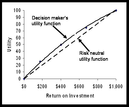
Figure 1: A risk seeking utility function
Sometimes, we have to estimate a utility function over an attribute that is not continuous or does not have a natural physical scale. For example, we might want to measure a utility scale (or in better words a disutility scale) over different types of skin diseases. In this approach, the worst and the best levels are fixed at 0 and 100 utilities. The decision maker is asked to come up with a probability that would make him indifferent between a new level in the attribute and a gamble involving the worst and best possible levels in the attribute. For example, suppose we want to estimate the utility associated with the following five skin diseases (listed in order of severity): No skin disorder, Kaposi's sarcoma, Shingles, Herpes complex, Candida or mucus, and Thrush.
The analyst assigns the best possible level a utility of 0. The worst possible level, Thrush, is assigned a utility of 100. The decision maker is asked to think if they prefer to have Kaposi's Sarcoma or a 90% chance of Thrush and 10% chance of no skin disorders. No matter what the response, the decision maker is asked the same question again but now with probabilities reversed: "Do you prefer to have Kaposi's Sarcoma or a 10% chance of Thrush and 90% chance of no skin disorders." The analyst points to the decision maker that the choice between the sure disease and the risky situation was reversed when the probabilities were changed. Because the choice is reversed, there must exist a probability at which point the decision maker is indifferent between the sure thing and the gamble. The probabilities are changed until a point is found where the decision maker is indifferent between having Kaposi's Sarcoma and probability p of having Thrush and probability (1-p) of having no skin disorders. The utility associated with Kaposi's Sarcoma is 100 times the estimated probability, p. A utility function assessed in this fashion will reflect not only the values associated with different diseases but decision maker's risk taking attitude. Some decision makers may consider a sure disease radically worst than a gamble involving a chance, even though remote, of having no disease at all. These estimates thus clearly reflect not only their values but their willingness to take risks. Value functions do not reflect risk attitudes. Therefore, one would expect single attribute value and utility functions to be different.
If preferential independence is met, several single attribute utility functions are aggregated into an overall score using additive or multiplicative summation rules. An additive multi-attribute utility function is commonly used in the literature. When the decision maker is assumed to be risk neutral, an additive multi-attribute utility function is mathematically the same as calculating an expected value.
A Summary Prepared by Jennifer A. Sinkule Based on Chatburn RL, Primiano FP Jr. Decision analysis for large capital purchases: how to buy a ventilator. Respir Care. 2001 Oct;46(10):1038-53.
It is sometimes helpful to introduce a hierarchical structure among the attributes, where broad categories are considered first and then within these broad categories, weights are assigned to attributes. By convention the weights for the broad categories add up to one and the weight for the attributes within each category also add up to one. The final weight for an attribute is the product of the weight for its category and the weight of the attribute within the category. The following example shows the use of hierarch in setting weights for attribute.
Chatburn & Primiano (2001) employed an additive, compensatory, multi-attribute utility model to assist the University Hospitals of Cleveland in their purchase of new ventilators for use in the hospitals’ intensive care units. A decision making model was useful in this instance because ventilators are expensive and complicated machines, and the administration and staff needed an efficient way to analyze the costs and benefits of the various purchase options, as even long-term equipment trials can be ineffective at identifying all the relevant strengths and weaknesses of a particular machine. The decision making model utilized input from relevant stakeholders regarding factors important to the decision to weigh the various purchase options. Each possible ventilator purchase was weighed according to the identified factors and ranked in terms of how well each option met each key decision factor. The model also provides an overall score which identifies the best purchase option, taken as a whole. The decision process began with an analysis of the hospitals’ current ventilator situation. Many factors suggested that the purchase of new ventilators would be advantageous. First, all of the ventilators owned by the hospitals were between 12 and 16 years old, while the depreciable lifespan of a ventilator is only 10 years. Thus, the age of the equipment put the hospitals at greater risk to experience equipment failures. Because ventilators are used primarily for life support, should this equipment fail the hospitals would be highly liable. Second, the costs to maintain the older equipment were beginning to outweigh the initial capital investment. Third, the current fleet of ventilators varied in age and model. Some ventilators could be used only for adults while others could only be used for infants or children, and different generations of machines ran under different operating systems. The result was that not all members of the staff were facile with every model of ventilator, yet it seemed impractical to invest in the type of extensive staff training which would be required to correct this problem. Therefore, the goals for the ventilator purchase were to advance patient care capabilities and increase staff competence, to reduce maintenance costs by acquiring ventilators which could be maintained via technical support updates and upgrades versus replacement of parts, and to reduce the capital inventory in order to lower both maintenance and staff training costs. To begin the selection process, the consultants wanted to limit the analysis to only the most relevant choices, those machines that were designed for use in intensive care units with an ability to ventilate multiple types of patients. In addition, it was important to select a company with good customer support and the availability of software upgrades. Also, as well as cost analysis, the analysis involved both a clinical and technical evaluation of each ventilator model. Each possible ventilator was used in the hospitals units on a trial basis for 18 months so that staff could familiarize themselves with each model. The technical evaluation utilized previously published guidelines for ventilators as well as vendor-assisted simulations of various ventilator situations so that administrators and staff could compare the functionality of the different models. A checklist was used in this instance to evaluate each ventilator in three major areas: control scheme, operator interface and alarms. Figure 1 depicts the attributes, their levels and relative weights used in the final decision model.
Figure 1: A Hierarchy for Assessment of Attribute Weights
Note that weights were first assessed across broad categories (cost, technical features and customer service). Two of these broad categories were broken into additional attributes. Weights for broad categories were assessed (note that these weights add up to one). In addition, the weights for each attribute within the categories were also assessed (note that these weights also add up to one within the category). In the end, the model had eight attributes in total and the weight for attributes was calculated as the product of the weight for broad category and the weight of the attribute within that category.
So how did this model perform in the real world? According to personal communication from the authors, there were two major problems experienced by the hospital staff. The first was reaching consensus on the weight of the cost factor. Ultimately, a more practical approach was to remove cost as a weighted factor and increase the weights of the remaining factors proportionately (i.e., technical features = 0.6 and customer service = 0.4.) Then, the score for each ventilator model was divided by its cost to give a more intuitively satisfying “benefit/cost” ratio. The second problem was more political than practical. Any rational decision can be based on only one of three strategies: (1) minimize cost, (2) maximize benefit, or (3) optimize the ratio of benefit/cost. In a hospital, physicians often have a large influence on purchase decisions when they argue from the standpoint of “what is best for the patient”, which usually ignores cost. Senior hospital administration, on the other hand, is usually more likely to base a decision on cost because they have to choose among many proposals competing for limited capital funds. Middle managers, like the authors of this paper, naturally sought a balance and took the benefit/cost approach. In the end, the physicians won out and the most expensive ventilator was purchased based on the perception that it provided the highest quality. As a result, the cost had to be spread out over 3 years with equal purchases of ventilators each year. Unfortunately, by the third year, funding for this project was no longer available. This shows how varied and unpredictable real-world factors can degrade an otherwise very logical decision process.
Construct a value function for a decision at work. Select a decision that does not involve predicting uncertain outcomes (e.g. see examples). Select an expert that will help you construct the model. Make an appointment with the expert and construct the model. Prepare a report that answers the following questions:
Prepare your report using narrated Power Point slides (SWF). Keep the following rules in mind in narrating a slide presentation:
Send your report to your instructor and at least one other student in class. Mail your report, do not email narrated slides (narrated slides take considerable space). Keep a copy for yourself till end of semester. Your instructor will ask for your entire portfolio of assignments at end of semester again.
The slide show should contain following slides:
Do not exceed 7 slides, do not exceed 2 minutes per slide. To see how the slide show will be graded, click here.
Here are example of work done by students (please note that these are not necessarily model projects):
To assist you in reviewing the material in this lecture, please see the following resources:
Listen to Modeling Preferences
See the slides for the lecture
See a video on how to create an X-Y diagram and correlations in Excel.
See a video on how to calculate correlations in Excel using Data Analysis Tool Pack
Narrated lectures require use of Flash.
Alemi F, Stokes J 3rd, Rice J, Karim E, LaCorte W, Saligman L, Nau R. 1987. "Appraisal of Modifiable Hospitalization Risk." Medical Care 25 (7): 582‑91.
Alemi, F., B. Turner, L. Markson, and T. Maccaron, 1990. "Severity of the Course of AIDS." Interfaces 21: 105‑6.
Alemi F, Walker L, Carey J, Leggett J. Validity of three measures of severity of AIDS for use in health services research studies. Health Serv Manage Res. 1999 Feb;12(1):45-50.
Aschenbrenner, K., and T. Kaubeck. 1978. "Challenging the Cushing Syndrome: Multi‑Attribute Evaluation of Cortisone Drugs." Organizational Behavior and Human Performance 22 (2): 215‑34.
Beach, L. R., F. L. Campbell, and B. D. Townes. 1979. "Subjective Expected Utility and the Prediction of Birth‑Planning Decisions." Organizational Behavior and Human Performance 24: 18‑28. See also Wood RJ, Campbell FL, Townes BD, Beach LR. Birth planning decisions. Am J Public Health. 1977 Jun; 67(6): 563-5.
Bernoulli, D. 1938. "Spearman theoria novai de mensura sortus." Comettariii Academiae Saentiarum Imperialses Petropolitica 5: 175‑92. Translated by L. Somner in Econometrica 22 (1954): 23‑36.
Cline, B., F. Alemi, and K. Bosworth 1982. "Intensive Skilled Nursing Care: A Multi‑Attribute Utility Model for Level of Care Decision Making." Journal of American Health Care Association.
Cook, R. L., and T. R, Stewart. 1975. "A Comparison of Seven Methods for Obtaining Subjective Description of Judgmental Policy." Organizational Behavior and Human Performance 12: 31‑45.
Detmer DE, Moylan JA, Rose J, Schulz R, Wallace R, Daly R.. 1977. "Regional Categorization and Quality of Care in Major Trauma." Journal of Trauma 17 (8): 592.
Edwards, W. 1974. "The Theory of Decision Making." Psychology Bulletin 51 (4): 320.
Edwards, W. 1977. "How to Use Multi‑Attribute Utility Measurement for Social Decision‑Making." IEEE Transactions on Systems, Man and Cybernetics SMC7: 326‑40.
Ericsson, K. A., and H. A. Simon, 1980. "Verbal Reports as Data." Psychological Review 87: 215‑51. See citations of this work.
Fischer, G. W. 1979. "Utility Models for Multiple Objective Decisions: Do They Accurately Represent Human Preferences?" Decision Science 10: 451.
Fryback DG, Gustafson DH, Detmer DE. Local priorities for allocation of resources: comparison with the IMU. Inquiry. 1978 Sep; 15(3): 265-74.
Gustafson, D. H., M. E. Hiles, and C. Taylor. 1980. "Report on the Trauma Severity Index Conference." Center for Health Systems Research and Analysis, University of Wisconsin‑Madison.
Health Services Research Group, Center for Health Systems Research and Analysis, University of Wisconsin. 1975, "Development of the Index for Medical Under‑service." Health Services Research 10 (2): 168‑80.
Hogarth, R. M. 1975. "Cognitive Processes and the Assessment of Subjective Probabilities." Journal of American Statistical Association 70: 271‑94,
Humphrey, S. P., and A. Humphrey. 1975. "An Investigation of Subjective Preference Orderings for Multi‑Attribute Alternatives." In Utility, Probability and Human Decision‑Making, edited by D. Wendt and C. Vlek, pp. 119‑23. The Netherlands: D. Reidel Publishing Co.
John, R. S., and W. Edwards. 1978. "Subjective versus Statistical Importance Weights: a Criterion Validation." Research report, Social Science Research Institute, SSRI 78‑7, University of Southern California.
Johnson, E. M., and G. P. Huber. 1979. "The Technology of Utility Assessments: Issues and Problems." IEEE Transactions in Systems, Man and Cybernetics. Kahneman, D., and A. Tversky. 1979. "Prospect Theory: An Analysis of Decisions Under Risk." Econometrica 47: 263‑91.
Kahneman, D., and A. Tversky. 1979. "Prospect Theory: An Analysis of Decisions Under Risk." Econometrica 47: 263‑91.
Kao, E. P. C. 1972. "A Semi Markov Model to Predict Recovery Progress of Coronary Patients." Health Services Research 7: 191‑208.
Keeney, R. 1980. "Analysis of Preference Dependencies among Objectives." Woodward and Clyde Consultants (July).
Keeney, R. 1977. "The Art of Assessing Multi‑Attribute Utility Functions." Organizational Behavior and Human Performance 19: 267‑310. See citations of this work.
Keeney, R. L., and H. Raiffa, 1976. Decisions and Multiple Objectives: Preferences and Value Tradeoffs. New York: John Wiley.
Kinzbrunner B, Pratt MM. Severity index scores correlate with survival of AIDS patients. Am J Hosp Palliat Care. 1994 May-Jun;11(3):4-9.
Kneppreth, N. P., D. H. Gustafson, and R. P. Leifer. 1974. "Techniques for Assessment of Worth." Technical Paper 254, U.S. Army Research Institute for the Behavioral and Social Sciences, Arlington, MD.
McNeil BJ, Pedersen SH, Gatsonis C. Current issues in profiles: potentials and limitations. In: Physician Payment Review Commission Conference on Profiling. No. 92-2. Washington, D.C.: Physician Payment Review Commission, 1992:46-70.
Naglie G, Krahn MD, Naimark D, Redelmeier DA, Detsky AS. Primer on medical decision analysis: Part 3--Estimating probabilities and utilities. Med Decis Making. 1997 Apr-Jun;17(2):136-41.
Nisbett, R., and L. Ross. 1980. Human Inferences. Englewood Cliffs, NJ: Prentice‑Hall.
Nisbett, R. E., and T. D. Wilson. 1977. "Telling More Than We Can Know: Verbal Reports on Mental Processes." Psychological Review 84 (3): 231‑59.
Pai, G. K., D. H. Gustafson, and G. W. Kiner. 1971. "Comparison of Three Non‑Risk Methods for Determining a Preference Function." Center for Health Systems Research and Analysis, University of Wisconsin‑Madison. See also Gustafson DH, Fryback DG, Rose JH, Prokop CT, Detmer DE, Rossmeissl JC, Taylor CM, Alemi F, Carnazzo AJ. An evaluation of multiple trauma severity indices created by different index development strategies. Med Care. 1983 Jul; 21(7): 674-91.
Pascal, A., C. L. Bennett, and M. C. Bennett. 1989. "The Cost of Financing Care for AIDS Patients: Results of a Cohort Study in Los Angeles." National Center for Health Services Research Conference Proceedings on New Perspectives on HIV‑Related Illness, NCHSR publications, Rockville, MD.
Pliskin, J. S., D. S. Shepard, and M. C. Weinstein. 1980. "Utility Functions for Life Years and Health Status." Operation Research 28 (1): 206. See also related articles.
Redfield, R. R., and D. S. Burke. 1988. "HIV Infection: The Clinical Picture." Scientific American 259 (4): 90‑98.
Rose W, Maffetone M, Suarez E, Whisler K, Bielitzki LD. A model for selecting a clinical laboratory information system. A four-phase process. Clin Lab Manage Rev. 1992 Jan-Feb;6(1):18-9, 22-4, 26-9.
Savage, L. D. 1972. Foundations of Measurement. New York: John Wiley.
Scitovsky, A. A. 1989. "Past Lessons and Future Directions: The Economics of Health Services Delivery for HIV‑Related Illness." National Center for Health Services Research Conference Proceedings on New Perspectives on HIV‑Related Illness, NCHSR publications, Rockville, MD.
Sessa EJ. Information is power: the Pennsylvania experiment. J Health Care Benefits 1992;Jan-Feb:44-8.
Snyder, M., and N. Cantor. 1979. "Testing Theories about Other People: Remembering All the History that Fits." Unpublished manuscript, University of Minnesota.
Torgerson, W. S. 1958. Theory and Methods of Scaling. New York: John Wiley.
VanGundy, A. B. 1981. Techniques of Structured Problem Solving. New York: Van Nostrand Reinhold.
Vibbert S. Illinois Blues target doctors. Medical Utilization Review. April 2, 1992.
Volkema, R. 1981. "Different Approaches to Problem Solving." Ph.D. thesis, University of Wisconsin.
Von Winterfeldt, D., and W. Edwards. 1986. Decision Analysis and Behavioral Research. New York: Cambridge University Press.
Warner, H. 1971. "Estimating Coefficients in Linear Models: It Don't Make No Never Mind." Psychological Bulletin 83 (2): 213‑14.
Yates, J. F., and C. M. Jagacinski, 1979. "Reference Effects in Multi‑Attribute Evaluations:" Organizational Behavior and Human Performance 24 (3): 400‑410.
Hawthorne G. The effect of different methods of collecting data: mail, telephone and filter data collection issues in utility measurement. Qual Life Res. 2003 Dec; 12(8): 1081-8.
Say, Rebecca E medical student 1. Thomson, Richard professor of epidemiology and
public health 2. The importance of patient preferences in treatment
decisions-challenges for doctors. BMJ. 327(7414):542-545, Accession
Number: 00002591-200309060-00031
(From the abstract) This article discusses the challenges faced by doctors who
are encouraged to involve patients in treatment decisions but must also consider
their own knowledge and evidence-based guidelines which may suggest a different
course of action. The authors call for innovative research and appropriate
professional training to find solutions to such problems, and discuss how
doctors might face the challenge of involving patients in treatment decisions.
Coffey, J. Todd, Brandle, Michael, Zhou,
Honghong, Marriott, Deanna Burke, Ray MA Tabaei, Bahman P. Engelgau,
Michael M. Kaplan, Robert M. Herman, William H. MD, MPH Valuing Health-Related Quality of Life in Diabetes.
Diabetes Care 25(12): 2238-2243, December 2002. Accession Number:
00003458-200212000-00020
(From the abstract) This article discusses the use of information on health
utilities by cost-utility analyses to compare medical treatments that have
different clinical outcomes and impacts on survival. The study presented
described health utilities associated with diabetes and its treatments,
complications, and co-morbidities.
Larrabee, June H. PhD, RN. Bolden, Lois V. RN, MSN. Knight, Marie Ray RN, MSN.
The lived experience of patient prudence in health care. Journal of Advanced
Nursing. 28(4):802-808, October 1998. Accession Number:
00004471-199810000-00040
(From the abstract) This article presents a study the purpose of which was to
describe the lived experience of patient prudence in health care. Prudence has
been defined as good judgment in setting realistic personal goals and using
personal resources to achieve those goals.
Gold, Marthe R. MD, MPH. Franks, Peter MD. McCoy, Kristine I. MPH. Fryback, Dennis G.
. Toward Consistency in Cost-Utility Analyses: Using
National Measures to Create Condition-Specific Values. Medical Care.
36(6):778-792, June 1998. Accession Number: 00005650-199806000-00002
(From the abstract) The authors present their development of an “off-the-shelf”
source of health-related quality of life scores for cost-effectiveness analysts
who are unable to collect primary data.
Nease RF Jr, Kneeland T, O'Connor GT, et al. Variation in patient utilities for
outcomes of the management of chronic stable angina. Implications for clinical
practice guidelines. Ischemic Heart Disease Patient Outcomes Research Team. JAMA
1995;273:1185. Accession Number: 00005407-199504190-00023
(From the abstract) This article investigates the potential importance of
patient preferences in the treatment of ischemic heart disease, as practice
guidelines often make recommendations based on symptom severity while rarely
accounting for how patients feel about their symptoms. To do so, the authors
assessed attitudes toward symptoms in patients with angina pectoris.
This page is part of the course on Decision Analysis, the lecture on Preferences. It was last edited on 05/12/2003 by Farrokh Alemi, Ph.D. © Copyright protected. This page is based on a chapter with the same name published by Gustafson DH, Cats-Baril WL, Alemi F. in the book Systems to Support Health Policy Analysis: Theory, Model and Uses, Health Administration Press: Ann Arbor, Michigan, 1992.