|
|
|||||||||||||||||||||||||||||||||||||||||||||||||||||||||||||||||||||||||||||||||||||||||||||||||||||||||||||||||||||||||||||||||||||||||||||||||||||||||||||||||||||||||||||||||||||||||||||||||||||||
Introduction to Probability ConceptsWe quantify the probability of an event so that we can make tradeoffs among uncertain events, measure the combined impact of several uncertain event and communicate our uncertainty about future events to others. Probability quantifies how uncertain we are about a future events. The best way to think of probabilities is as the ratio of all ways in which an event may occur divided by all possible events. In short, probability is the prevalence of the event of interest among the possible events. The probability of you exercising 30 minutes a day is the number of days in which you exercised 30 minutes divided by the total number of days examined. Lets say we keep track of your exercise for 2 weeks and during this period you exercised 5 days, then the daily probability of exercise is 5/14=0.35. If we were only planning to exercise during the weekdays, then the daily probability of exercise during week days is 5/10=0.50. Many find it easier to express probability as the percent of total possible events. For example, instead of saying that the probability of exercising during week days is 0.50, we can state that we exercised in 50% of week days. Both statements are equivalent. Probability numbers range from 0 to 1, while the percent numbers range from 0% to 100%. When we are sure that an event will occur, we say that it has a probability of 1. When we are sure that an event will not occur, we assign it a probability of zero. When we are completely in dark, we give it a probability of 0.5, a fifty - fifty chance of occurrence. All other values between 0 and 1 measure how uncertain we are about the occurrence of the event. Please note that this definition of probability leads to the following conclusions, which are typically referred to as the axioms of probability:
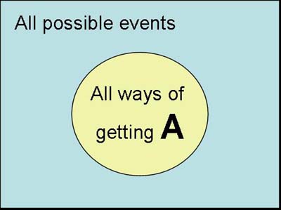
A useful way to understand probabilities is to get a visual intuition about it. A Venn diagram shows the frequency of an event compared to the frequency of all possible events. The circle in Figure 1 shows the frequency of event A and the rectangle shows the frequency of all possible events. The blue portion of the rectangle shows the frequency of events that are "not A". Note how the sample space is the sum of the event and its complement. This is implied by the 1st and 3rd axioms. The first axiom requires the probability of the entire sample to be one. The third axiom requires that probability of the complement to be one minus probability of the event.
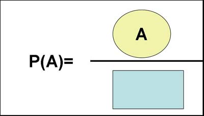
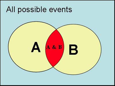
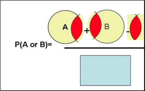
Figure 1: A Graphical Intuition for Definition of Probability Using our definition, the bottom part of Figure 1 shows the probability of A is the circle representing all occasions in which A occurs divided by the rectangle representing all possible events. So what is the probability of "not A." Graphically, it is all the blue area with the hole in the middle divided by the rectangular area. Logically it is the count of all events that are "not A" divided by all possible events. So what is the probability of exercising? It is the count of days in which we exercised divided by total days. What is the probability of not exercising? It is the count of days in which we did not exercise divided by total days. Note that the sum of probability of exercising and not exercising will always be 1 as these two events are mutually exclusive (in any day, one is either exercising or not exercising) and exhaustive (no other events are possible besides these two). Probability of Combination of EventsThe rules of probability allow us to calculate probability of combination of events. The probability of two events A and B occurring together, is calculated by first summing all the possible ways in which event A will occur plus all the ways in which event B will occur, minus all the possible ways in which both event A and B will occur (this term is subcontracted because it is double counted). The numerator is divided by the all possible ways that any event will occur. This is represented in mathematical terms as: P(A or B) = P(A) + P(B) - P(A & B) Graphically, the concept can be shown as the yellow and red areas in Figure 2 divided by the blue area.
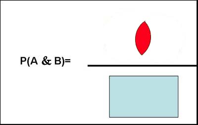
Figure 2: Graphical Representation of Probability of A or B Similarly, the probability of A and B occurring together, corresponds to the overlap between A and B and can be shown graphically as the red area divided by all possible events (the rectangular blue area) in Figure 3.
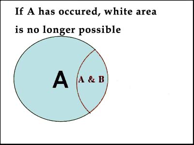
Figure 3: Graphical Representation of Probability A and B The definition of probability gives us a simple calculus for combining uncertainty of two events. We can now ask questions such as: "What is the probability that you would exercise in the morning or in the evening?" According to our formulas this can be calculated as: P( Exercise in morning or evening) = Since the chance of exercising in both the morning and evening is almost nil, we can re-write the formula as: P( Exercise in the morning or evening) = P( Exercising in morning) + P(Exercise in the evening) As you can see, the calculus of probability gives us a simple formula for examining either of two events occurring, specially when the chances of both events occurring is near zero. Measuring Impact of a CauseThe impact of a cause is measured through conditional probability, where the probability of the effect is reported given when the cause is present. Recall that we defined probability as the count of occasions in which an event occurs divided by all possible events. This definition also helps us calculate the probability of an event conditioned on the occurrence of other events. In these circumstances, we know something (e.g. the cause) has happened and we are asking for the calculation of the probability of an event (typically the effect). In mathematical terms we show this as P(A | B) and read it as probability of A given B. When an event occurs, it reduces possibilities; we no longer need to track the possibility that the event may not occur. The universe of possibilities shrinks. To calculate conditional probability we need to merely keep track of the shrinking universe of possibilities. We need to restrict the possibilities to only events that are now possible. Graphically, this is shown as in Figure 4.
Figure 4: Probability of B Given A is Calculated by Reducing Possibilities In the top of Figure 4, the white space is no longer possible as the event A has occurred and nothing outside the blue area is any longer possible. Therefore the rectangular universe of possibilities has shrunk to the circle representing event A. In the bottom of Figure 4, this information is used to calculate the probability of B occurring given that A has occurred. The red sliver, the numerator on top of the equation, designates all occasions in which B might occur and the blue circle in bottom of the equation, the denominator, shows all possible events (all of which include event A occurring). Another way of saying this is that the conditional probability of the effect given the cause is calculated as follows:
Or similarly: p(Effect | Cause) = p(Effect & Cause) / p(Cause) For example, suppose we want the probability of exercise given that we sleep early at night. The idea seemed simple, do not watch late shows, get up early and exercise. Now we are interested to know if this is working out. We need to calculate the conditional probability of exercise given sleeping early. In this example, the red sliver, the numerator on top of the equation, is the number of days in which we exercised in the morning and slept early. This represents both the cause and the effect occurring. The denominator, at the bottom of the equation, is the total number of days in which we slept early. This represents the number of times the cause was present. The impact of sleeping early on probability of exercise is the ratio of the two numbers. Let us do a numerical example. In Table 1, the joint probability of sleeping early and exercising is calculated from number of days we slept early and days we exercised. The probability of each event is calculated by dividing the frequency of the event by 30, the total number of days. The probability of morning exercise is17, the total number of days in which we exercised in the morning, divided by 30 or 0.56. Now, we need to calculate the probability of morning exercise given that we sleep early. We start by shrinking the universe to the condition within the conditional probability statement, i.e. sleeping early. The reduced universe of possibilities is 27 days in which we slept early. This is the number of days the cause was present. Among the days in which we slept early, there were 15 days in which we exercised, this is the joint occurrence of the cause and the effect. This is the count of exercise in the reduced universe of possibilities. The conditional probability is calculated as 15 divided by 27, which is 0.55: p(Exercise | Sleep early) = Number of days of both sleeping early and exercise / Number of days of sleeping early = 15 / 27 = 0.55 Our probability of exercise does not seem to change. Therefore, our assumption that sleeping early is helping us exercise is not supported.
Since Table 1 provides the count as well as the probabilities, we can describe the above calculations in terms of probabilities: p(Exercise | Sleep early) = P(Both exercise and sleeping early) / p(sleeping early) = 0.51/ 0.90 = 0.55 The point of this example is that conditional probabilities can be calculated easily by reducing the universe examined to the condition within the conditional probability. You can calculate conditional probabilities from the count of events or from the probabilities of remaining events if you keep in mind how the condition has reduced the universe of possibility. Conditional probabilities are a very useful concept. They allow us to think through an uncertain sequence of events. If each event can be conditioned on its predecessor, a chain of events can be examined. Then if one component of the chain changes, we can calculate the impact of the change through out the chain. In this sense, conditional probabilities show how a series of clues might forecast a future event. Impact of Multiple CausesThe analysis described in the previous section can be carried out for multiple causes. Table 2 shows an example set of data. This example shows the type of data usually available from a causal diary (a diary in which the person tracks both the cause of the behavior and the behavior).
The Table lists two causes (sleeping early and planning with buddy) and tracks every day whether the person succeeded in exercising. The question of interest is which of these causes predict the exercise outcome best. To answer this question, we need to calculate the conditional probability of exercise given each of the two causes (in later lectures we show how the calculation of conditional probabilities needs to be modified to reflect the co-occurrence of the two causes but for now we are assuming that the impact of each cause is independent of the other). The process of calculating conditional probability follows the procedures described in the previous section, i.e. first we restrict the data to the situation where the cause has happened and then we report the frequency of the effect divided by the number of times the cause has happened. To see this, lets start with analysis of the impact of planning with a buddy. First we restrict the data to all occasions in which we had made plans with a buddy. Table 3 shows the result.
Now we can count how many times we exercised (8 times) and how many days we had planned with our buddy. The conditional probability of exercise given planning with the buddy is the ratio of these two numbers: p(Exercise | Planning with buddy) = 8/8 = 1 In 100% days in which we had plans to exercise with a buddy, we did in fact exercise. Now we can try the same procedure for calculating the conditional probability of exercise given sleeping early at night. We start with the original diary data and again restrict the dataset to all cases in which the condition is met, in this case days in which the night before we had slept early. Table 4 shows the result:
Table 4 shows that there were 9 days in which we had slept early the night before. Among these days we exercised on 5 days. Therefore the conditional probability of exercise given sleeping early the night before is: p(Exercise | Sleeping early) = 5/9 = 0.56 Based on this analysis it seems that planning with a buddy is more likely to lead to exercise than sleeping early. The analysis we have done is flawed in an important way. Sleeping early and planning with a buddy co-occur 37% of time. In these time periods we do not know if the impact on probability of exercise is due to sleeping early or planning with a buddy. In a later lecture we show how to adjust calculation of conditional probability of effect given a cause to reflect the co-occurrence among the causes. Some people prefer to describe their uncertainty about an event in terms of odds for the event occurring and not use the concept of probability. The two concepts are related. Odds are expressed as ratios while probabilities are expressed as decimals between 0 and 1. The odds for an event is related to its probability by the following formula:
For example, if the probability of an event is 90%, the odds for it is 0.9/(1-0.9) = 9 to one. If the odds of an event is 2 to one, the probability for the event is 2/(1+2) = .66. Odds and probabilities are always positive numbers. There is no upper limit to an odd ratio but the maximum probability is 1. An odds of 1 to 1, implies a 50% chance or a probability of 0.50. This shows that the person is completely uncertain about the event. Odds of 2 to 1 increase the probability of the event to 0.66. Odds of 3 to 1 increases the probability of the event to 0.75 and odds of 4 to 1 increases the probability of the event to 0.8. Sources of DataThere are two ways to measure probability of an event.
Both methods produce probabilities, but one approach is objective and the other is based on opinions. Both approaches measure the degree of uncertainty, but there is a major difference between them. Objective frequencies are based on observation of the history of the event, while measurement of strength of belief is based on an individual's opinion, even about events that have no history (e.g. what is the chance that you will exercise if you start a new job.) Savage (1954) and DeFinetti (1964) argued that the rules of probabilities can work with uncertainties expressed as strength of opinion. Savage termed the strength of a decision maker's convictions "subjective probability" and used the calculus of probability to analyze them. Subjective probability can be measured along two different concepts: (1) intensity of feelings and (2) hypothetical action (Ramsey 1950). One can measure subjective probability on the basis of intensity of feelings by asking about the hypothetical frequency that the event will occur. Suppose we want to measure the probability that we will exercise in the new job. Using the first method, we would ask:
When measuring according to hypothetical frequencies, we ask:
If both the subjective and the objective methods produce a probability for the event, then obviously the calculus of probabilities can be used to make new inferences from these data. But how can we argue that subjective probabilities measured as intensity of feelings should be treated as probability functions? To answer this, we must return to the formal definition of a probability measure. A probability function was defined by the following characteristics:
These assumptions are at the root of all mathematical work in probability, so any beliefs expressed as probability must follow them. Furthermore, if these three assumptions are met, then the numbers produced in this fashion will follow all rules of probabilities. Are these three assumptions met? The first assumption is always true, because we can assign numbers to beliefs so they are always positive. But the second and third assumptions are not always true, and people do hold beliefs that violate them. We can, however, take steps to ensure that these two assumptions are also met. For example, when the estimates of all possibilities (e.g., probability of success and failure) do not total 1, we can standardize the estimates to do so. When the estimated probabilities of two mutually exclusive events do not equal the sum of their probabilities, we can ask whether they should, and adjust as necessary. In your thinking, you may not follow the calculus of probability. But what you do and what you should do are two different issues. You may wish to follow the rules of probability, even though you have not always done so. Your opinions may not follow the rules of probability but you agree with the three principles listed above, then such opinions should follow the rules of probability. Our argument is not that probabilities and beliefs are the identical constructs, but rather that probabilities provide a context in which beliefs can be studied. That is, if beliefs are expressed as probabilities, the rules of probability provide a systematic and orderly method of examining the implications of these beliefs. Your subjective opinions about conditional probability of an effect given the cause tells you what you think. The objective frequency calculated from your diary tells you what it should be. By going back and forth over what you believe and what you should believe, you can correct your misconceptions about the impact of various causes. This page is part of the course on Lifestyle Management This page was last edited on 09/08/08 by Farrokh Alemi, Ph.D ©Copyright protected. |
|||||||||||||||||||||||||||||||||||||||||||||||||||||||||||||||||||||||||||||||||||||||||||||||||||||||||||||||||||||||||||||||||||||||||||||||||||||||||||||||||||||||||||||||||||||||||||||||||||||||