|
|
||||||||||||||||||||||||||||||||||||||||||||||||||||||||||||||||||||||||||||||||||||||||||||||||||||||||||||||||||||||||||||||||||||||||||||||||||||||||||||||||||||||||||||||||||||||||||||||||||||||||||||||||||||||||||||||||||||||||||||||||||||||||||||||||||||||||||||||||||||||||||||||||||||||||||||||||||||||||||||||||||||||||||||||||||||||||||||||||||||||||||||||||||||||||||||||||||||||||||||||||||||||||||||||||||||||||||||||||||||||||||||||||||
Self Experimentation and Causal ModelsA thinking Person's Guide to ExerciseThis lecture discusses how you can create a causal
model of your exercise habits. This lecture is based on, and at times
quotes verbatim from,
Alemi F, Moore S, Baghi H. Self-experiments and analytical relapse
prevention. Qual Manag Health Care. 2008 Jan-Mar;17(1):53-65. This
research was funded by Grant RO1 HL 084767 from the National Heart Blood and
Lung Institute.
Abstract
You may have many reasons why you do not exercise; you might list various causes or constraints; but research shows that many of these causal attributions are wrong. To help you gain insights into your own behavior, we suggest that you make a causal model of what you think influences your behavior. Then maintain a causal diary (a diary where in addition to recording successes or failures you also record the causes for these events). To start the diary, you make a list of causes of success and constraints that affect your behavior. Then you engage in thought experiments to verify the reasonableness and completeness of the list. Using the list, you keep a diary. At end of two to three weeks, the diary data are analyzed to find out the relationship between various causes as well as the relationship between the causes and exercise. A key issue in the analysis of diary data is to separate out the effect of various causes. Typically causes co-occur making it difficult to understand their independent effects.
Introduction
When you want to change, occasionally you fail and relapse into old habits. In these circumstances, it is important to understand causes of relapse so that you can address the root cause of the problem. Like many others, you may focus on your motivation and not on the events and routines that have lead to the relapse. As a result, relapses reoccur and you fail to maintain your resolution. This lecture is organized to improve your understanding of root causes of your own behavior so that you can transcend the cycles of resolving to do something only to find out that you have failed to accomplish your resolution. You may give many excuses for why you have not kept up with your exercise plans, some of which are legitimate reasons. Unfortunately, research on relapse prevention shows that most people are likely to be wrong. The reasons they give for why they exercise does not predict their behavior. In short, they have a distorted view of why they fail to exercise and therefore are unlikely to find a way out of their predicament. They are unlikely to find a way out of making resolutions, changing for sometime and then relapsing to old behavior. Relapse prevention is widely practiced in substance abuse treatment, smoking cessation programs, treatment of depression, treatment of sexual dysfunctions and many more behavioral disorders (Jaffe, 2002; Larimer, Palmer, Marlatt 2005; Kadden 1996; McKay 1999). In almost all of these circumstances, when the clients who failed to keep up with their resolution make wrong causal attributions (Cherpitel, Bond, Ye, Borges, Room, Poznyak, Hao, 2006; Billing, Bar-On, Rehnqvist 1997; Ladd, Welsh, Vitulli, Labbe, Law 1997). The most egregious of these fallacies is a tendency to attribute success to your skills/efforts and failures to event outside of the client's control (Ahn, Kalish, Medin, Gelman 1995; Green, Bailey, Zinser, Williams 1994; Kinderman, Kaney, Morley, Bentall 1992). This lecture shows you how to check the accuracy of causal attributions you make. Investigation may reveal root causes that are surprisingly hidden and seemingly unrelated to the targeted behavior. A client with substance abuse disorder, for example, may fail to keep their resolution because their depression is not adequately controlled by their antidepressant. Instead of focusing on their medication, the client and the client's clinicians are likely to focus on client's motivation. In the end, the root cause remains unchanged and despite heroic effort, the client relapses to drug use. For another example, a person had resolved to lose weight but repeatedly failed to accomplish it and continued to eat "junk" food. He achieved his goal when he joined a car pool. How could a car pool reduce junk food? The car pool made him get home earlier and thus could prepare a meal, eat it, digest it and fall asleep earlier. These are surprising causal effects, the relationship between these causes and their effects are not always self apparent. Analysis is needed to reveal true causes of behavior. What is to be done?The steps in conducting a causal analysis of your behavior include the following:
Each of these steps are further explained in the following sections. Step 1: Comprehensive list of causes and constraintsA cause is defined as an event that leads to successful accomplishment of your resolution. Taking your morning shower in the gym could be a cause of exercise. Biking to work could be another cause of exercise. These two are changes in daily routines that can cause increased exercise. A constraint is an event that prevents a cause from occurring, e.g. rain prevents you from biking to work. As we have reviewed elsewhere causes and constraints must meet the following criteria:
A comprehensive list of causes and constraints includes all reasonable causes and constraints that might affect your target behavior during a specific time, usually 2 weeks. For example, one might list the following three causes:
In addition, rain might interrupt the ability to bike to work and therefore is added as a constraint. Table 1 summarizes how each of these causes or constraints meet the criteria for a reasonable causal event.
Step 2: Make a causal modelIn this step, you make a causal model of your behavior. A causal model has three equivalent presentations: the real world relationships (something we cannot capture without reducing events to other descriptions), a visual network presentation of causes and effects and a probability distribution of cause and effect. The latter two are the abstract representation of the real world relationships. One could deduce either the probability description or the network description from the other, i.e. that any visual element has an equivalent probability implication. Knowing one can produce the other. To create a visual display of a causal model, follow these steps:
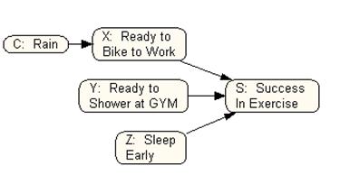
Using the information in Table 1, for example, we obtain the following causal model:
It shows that rain is a constraint on biking to work, preparation for biking to work, preparation for showering at gym and sleeping early are causes of exercise. For the purpose of ease of tracking the events, each event is also identified by a symbol: C for the constraint of rain, X for biking to work, Y for being ready to shower at gym, Z for sleeping early and S for success in exercising. In the example provided there are no relationships between various causes, i.e. we do not expect that on days in which we prepare to bike to work we need to sleep early, or that on days in which we prepare to bike to work we do not need to prepare to shower at the gym. If these assumptions were wrong, then an arrow should be drawn between the causes that are dependent. Furthermore, note that the causal model we have described is a-cyclical, meaning that we can not start at one point in the network, follow the arrows and arrive at the same point. A causal model is typically drawn without a cycle because we assume that the effect does not change the causes. This may not be true for all situations but for many, this is true. If there is a cycle, one can imagine model the first success in target behavior, thus breaking the cycle into several time-stamped returns to exercising. Every causal network structure has an equivalent probability statement. This allows us to draw a causal model and test its assumptions against observed data. A causal model is turned into probability model using conditional probability statements. Each node in the graph is calculated from the conditional probability of all links pointing to it. For example, the probability of exercise in the Figure 1 is measured as follows: p(Exercise | Ready to bike, Ready to shower at gym, Sleep early)= high p(Exercise | Ready to bike, Ready to shower at gym, Slept late)= Between low and high p(Exercise | Ready to bike, No plans to shower at gym, Sleep early)= Between low and high p(Exercise | No plans to bike, Ready to shower at gym, Sleep early)= Between low and high p(Exercise | Ready to bike, No plans to shower at gym, Slept late)= Between low and high p(Exercise | No plans to bike, Ready to shower at gym, Slept late)= Between low and high p(Exercise | No plans to bike, No plans to shower at gym, Slept late)= Low
Any event not depicted in the graph or depicted in the graph but not linked to the effect, does not affect the probability of the effect . So looking at Figure 1, the time we eat breakfast is not depicted and therefore it has no effect on exercise. Rain is depicted but it has an indirect effect through restricting biking to work on exercise.
In addition, a causal network shows a number of assumptions about probabilistic independence. For any two nodes linked to each other, the two are dependent. If not linked together, meaning if it is not possible to start from one and go to the other, the two events are independent. In probability distributions, two events are independent if the information about one event does not change the probability of the other. In probabilistic terms we show this as:
p(A |B) = p(A)
We read this as the probability of event A given event B is the same as the probability of event A. This statement says that knowing that event B has occurred does not change the probability of event A. If there are three nodes in the graph, more complicated independence statements must hold. The three most important independence statements for a three node graph or for any three nodes within a graph are the following:
As you can see, the way we draw the graph has implications for probability distribution and independence of events from each other. These implications can be verified through analysis of diary data as well as through thought experiments, a topic which we turn to next. Step 3: Construct Thought ExperimentsBefore proceeding to verify the accuracy of your causal assumptions against data, you need to test how consistent are various assumptions you have made. You might draw a set of causes as independent from each other but change your mind after you think through the events. You have to see if all the implications of the model you have produced are reasonable through the following tests:
Table 2 summarizes the thought experiments we carried out on our model of causes of exercise:
Though experiments help you look at the implications of causal relationships and see if the assumptions for these relationships are met. Through this step, you can make a number of modifications in the list of causes and constraints further focuses on events that affect your behavior. Step 4: Maintain a Causal DiaryA diary is a daily record of your success and failure. A causal diary is slightly different. In addition to recording whether you succeeded or failed, you also keep track of the causes or constraints that were present on that day. The key to a causal diary is to start with a list of causes and failures that is as comprehensive as possible and to indicate on each day which of these causes or constraints were present. Figures 2 and 3 show a diary designed for monitoring causes and barriers to exercise. The diary has two pages: A daily page to capture what happened on a particular day and a back page, half of which shows when looking at the daily page and lists possible causes imagined by the client. Figure 2 shows the daily page:  Figure 2: A Sample Daily Diary Page for Exercise The back-page includes a Fishbone Diagram to assist the client in thinking through various causes of their behavior. On the right of the page, clients can list the key causes they want to monitor for the next 2 weeks. The creation of a list of causes to track is done prior to start of the diary entries. This section of the back-page can be seen when looking at the daily page. Figure 3 shows a sample back page organized for listing causes of exercise:  Figure 3: A Sample Diary Back Page for Exercise The causal diary is used for 2-3 weeks to monitor the occurrences of causes listed in the back page. Moore and Alemi (2007) are using the diary described in Figures 2 and 3 to help patients who have had a cardiovascular event to return to exercise. You can create a causal diary that is easy for you to track. It could be simply a Table such as Table 3.
Step 5: Analyze dataThe analysis of diary starts with a few house keeping tasks. Sometimes, you may list causes that are so rare that they never occur during the 2-weeks diary period. These causes are not included in the analysis. Other times, two causes always co-occur with each other in every data entry. These two causes cannot be distinguished through data analysis and a new cause that reflects the combination of the two is defined and used in the analysis. For simplification we assume that only main effects of causes are of importance to us and interaction among causes can be ignored -- except for interaction between a constraint and a cause. The structure of Bayesian network is now relatively simple. Either the cause is directly affecting success rates or the combination of the cause and the constraint are affecting success rates. This simplification ignores positive interactions among two causes. As we will see shortly, to the extent that these interactions exist, it will lead to wider range of parameters estimated for the Bayesian Network. One way to estimate the conditional probability of success given the various causes is to limit the data to the cases in which the cause has occurred and is not limited by any constraints. We refer to these occasions as unconstrained causes. Then the conditional probability of success given the cause is calculated as the frequency of success among occasions of unconstrained causes. For example, to calculate p(S|X) we first restrict the cases to all situations where unconstraint causes are present and then calculate p(S) in this reduced sample space. This produces a maximum estimate for the impact of the cause on success as it assumes all successes reported in the reduced sample space did not have an alternative cause.
For a minimum estimate of the impact of the cause on success rate, all successful cases with alternative causes are ignored and the frequency of success re-calculated. This procedure of calculating maximum and minimum estimates for the conditional probability of success given a cause takes into account the co-variation among the causes.
Note that this method of analysis ignores the relationship among the causes. These relationships affect the minimum and maximum probability of success given the cause. Thus, despite the fact that we do not formally include cause-cause interactions in our model, the estimates of conditional probabilities are affected by potential cause-cause interactions. Suppose you have collected the diary data in Table 2. You had hypothesized three causes of exercise In Figure 1.. First cause was if planning to bike to work leads to exercise. The second cause was if planning to take morning showers in the gym, would increase visits to the gym. The last possible cause was to sleep early and thus be able to wake up earlier and have more time in the morning. The diary also marks rainy days, which are expected to reduce the possibility of biking to work.
Note that rainy day is assumed to affect “biking to work.” The first step in the analysis is to change the marker for biking to work to "No" when ever it rained and it was not possible to bike. The adjusted data are shown in Table 3.
Using the adjusted client's data in Table 3, you can calculate the maximum and minimum conditional probability of success for various causes. Table 4 shows the reduction of diary entries if you look at days in which you were planning to bike to work and it was not raining.
From this table we can note that in all days in which the client was ready to bike, the client did exercise. Therefore, the maximum probability of success given the plan to commute by bike is: P(S | Plan to commute) Max =1.0 The minimum probability of success is obtained by eliminating days in which alterative explanations are possible. This includes day 4 as on this day the plan to shower at the gym might have led to exercise. Therefore the minimum probability of success is calculated solely based on the data in day 14 and is: P(S | Plan to commute) Min =1.0 Table 5 shows the calculation of maximum and minimum probabilities of success on days in which you were ready to take shower at the gym.
Table 5 shows that the client exercised on 6 out of 7 days in which she was ready to take a shower at the gym: P(S | Ready to Shower at Gym) Max = 0.86 Some of these exercise patterns might be due to other causes. Of the 7 days, alternative explanations of causes of exercise exist for day 2 and day 4. Note that on day 3 we do have an alternative explanation but no success and therefore there is no reason to delete this day. If day 2 and 4 are dropped from analysis then there are 5 days in which we planned to shower at the gym and had no other alternative reason for exercise. The probability of success in this reduced space is 4 out of the remaining 5 days. Therefore the minimum estimate for the probability of success given that we are ready to shower is given as: P(S | Ready to Shower at Gym) Min = 0.80 Table 6 shows the maximum and minimum probability of success associated with each cause.
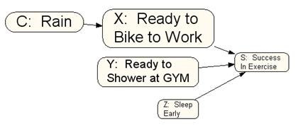
Step 6: Taking actionThe analytical process of thinking through causes of exercise and listing them by itself is beneficial. It leads to new insights. The thought experiments we presented earlier help you understand what might be a false cause. At some point, you arrive at a list of reasonable causes and constraints, then a 2-3 week of data collection help you sort out which of the causes are the most influential one. Through out this process you gain insight into what is keeping you from success and what is enabling you to move forward. It maybe helpful to represent the impact of causes on success visually (the font size is altered to reflect the magnitude of the conditional probability of success given the cause). We have done so in Figure 4.
Figure 4:
Causal Model with Font Size Reflecting Strength of Causes Keep in mind that the purpose of putting numbers on the impact of causes is to help produce insights. The focus should be on improvement and not measurement. The data are presented without any blame or exhortation for more effort. The purpose is to understand how the environment affects exercise and not to put more effort or be more motivated. Also keep in mind that any analysis is limited, You could not possibly look at all causes. At best you have focus on a handful of causes. Furthermore, the cause of your behavior may change over time. Given these limitations, the resulting analysis should be used with caution. If you do not jump to unsupported conclusions, some information is better than no information at all. After you gain insight into causes and constraints on your behavior, then act to enable the causes and remove the constraints (if that is possible). Continue with your data collection and see if the changes you have introduced, a quasi-experiment, have in fact increased the probability of success. DiscussionDiary data are observational data. To truly understand the impact of a cause on target behavior, we need experimental data. In experiments, one modifies a cause and observes if the probability of the effect is enhanced. Some scientists have suggested that in order to better understand the impact of different causes on your success or failure, you should use a full factorial experimental design (Olsson, Terris, Elg, Lundberg, Lindblad 2005). In a full factorial design all possible combination of causes are tried to see which one has the desired effect. This approach allows statisticians to estimate the main and interaction effects for various combinations of causes. Alemi and Alemi (2007) point out that a full factorial design is not practical as it will require clients to continue their experimentation even after they have found initial success in one of the trials. Most people would stop experimentation after they succeed. If they find a cause that makes them change their target behavior they do not and should not continue with the experimentation for finding the impact of other causes. Because they do so, only a partial factorial design will be available and main effects of causes maybe confounded with higher order interactions among the causes. Instead of having a design that will sort out the effect of various causes, most people collect observational data that are often correlated and difficult to analyze. The problem is made more intractable because of the limited amount of data collected in a diary. For example, over 2 weeks of keeping an exercise diary, assuming that the you have been faithful and made an entry every day, there is a total of 14 data points -- from which you need to estimate a large number of parameters. When there are 3 causes, there are 3 main effects, 3 pair-wise interactions, and 1 three-way interaction. This is a total of 7 parameters that must be estimated. With 4 causes, there are 4 main effects, 6 pair-wise interactions, 4 three-way interactions and 1 four-way interaction. With 5 causes there are 5 main effects, 10 pair-wise interactions, 10 three-way interactions, 5 four-way interaction and 1 five-way interaction. In general, if there are n causes and interactions of k causes are to be considered, then there are n!/(n-k)!k! possible interactions. Obviously, when many causes are considered, the number of parameters that must be estimated often exceeds the number of data points available. One way out of this shortage of data is to focus on estimating the main effects and ignore all interactions, as we have done in this lecture. But some interactions, in particular constraints on a cause, could completely change the situation. Ignoring these constraints will distort the estimated main effects of causes. For example, a cause leading to exercise is “planning to commute to work by biking.” “Rain” might be a constraint on the impact of this cause, meaning the client will not bike to work if it is raining. Ignoring the impact of this constraint will not make sense as rain does not reduce the impact of the decision to bike to work on exercise levels by a few points, it completely eliminates it. In this paper, we show an algorithm that ignores most interactions but not the interactions between causes and constraints. Traditional statistical methods (e.g. Analysis of Variance) are not useful in
analysis of diary entries because there are many parameters to estimate and
there are many potential associations among combination of causes.
Instead, we rely on artificial intelligence and heuristic methods of learning
from a small sample of cases. In particular, we rely on progress made in
Causal Modeling and Bayesian Networks ( Building a causal model requires learning the model structure and parameters from the diary data. Unfortunately, as mentioned earlier, diary data is limited. In most cases, patients are asked to collect information on factors that may change in 2-3 weeks. This yields between 14 to 21 data points, from which both the structure and the parameters of the Bayesian Network must be assessed. Heckerman et al (1999) have shown that with samples of size 500, significant errors in detecting the structure of Bayesian Networks could occur. With sample size of 14, a great deal more errors can occur. To remedy the lack of data, we use client’s insight into the problem to guide the learning of Bayesian Network structure. This is different from un-guided machine learning typically done for learning structure of Bayesian Networks (Neapolitan 2004). To begin with, we know that causes lead to effect and not vice versa. The client has specified the causes that positively affect exercise. This specification also removes the possibility of a directed link from exercise to the cause. Furthermore, we know that the client has expressed the constraints that would remove the cause from consideration. In our terminology, a cause increases probability of exercise and a constraint reduces probability of exercise through removing the positive effect of a cause. Anecdotal data suggest that clients can express causes and constraints with ease. Since the client has specified which constraints work on which cause, this information too can be used to construct the links in the network. This lecture has provided an approach to analyzing causes of your behavior using observational data from a diary. The expectation is that a focus on causes of your behavior can help you create an environment where you are more likely to keep with your plans and achieve your resolution. The hope is that out of the emerging understanding will come a new situation where you will succeed despite your wavering motivation. References
This page is part of the course on Lifestyle Management This page was last edited on 09/08/08 by Farrokh Alemi, Ph.D ©Copyright protected. |
||||||||||||||||||||||||||||||||||||||||||||||||||||||||||||||||||||||||||||||||||||||||||||||||||||||||||||||||||||||||||||||||||||||||||||||||||||||||||||||||||||||||||||||||||||||||||||||||||||||||||||||||||||||||||||||||||||||||||||||||||||||||||||||||||||||||||||||||||||||||||||||||||||||||||||||||||||||||||||||||||||||||||||||||||||||||||||||||||||||||||||||||||||||||||||||||||||||||||||||||||||||||||||||||||||||||||||||||||||||||||||||||||