Thank You

Thank you for submitting your data.  This page provides you with correct responses to selected assignments.

Presentation issues

A correction is needed if any of the following is present:

1. The chart includes un-named labels such as "Series 1" and "Series 2."
2. The markers in the control lines were not removed.
3. The chart does not have a title
4. The X-axis does not have a title
5. The Y-axis does not have a title
6. The chart is not easy to find.
7. Colors used in the chart and in the cell values, do not help in understanding of the work.
8. Except for the data, all cell values should be calculated as a formula.  If this is not the case, it is very important that you point this out.  You should be able to change a data value and all calculations should change automatically.

Accuracy

The chart should look like the following:

Figure 1;  Control Chart for the Assignment

First notice the feel and look of the chart:

1. Notice that the markers are removed from the UCL and LCL.  They are shown as lines as we want to attract attention to them as a line of limits across time.  In contrast the markers are shown in the observed rate line because we want to make sure that it is looked at as individual observations each time period.
2. Notice that Observed rate and not the expected rate is plotted.  Many students plot the expected rate, which will always be within limits and will not be informative.
3. Notice that both the X-axis and the Y-axis are labeled
4. Finally notice that the legend is available for the lines drawn in the chart.  None of the items in the legend is marked as "Series 1" or some other automated text that does not make sense in this context.

Check that the Expected Deviation was calculated correctly.  The following shows the necessary calculations.  I calculated the Expected Deviation by multiplying each patients' risk factor with one minus the patients' risk factor.  This is what I got:

Please notice that there are different number of patients in each time period.  When you copy and paste the formula, make sure that the student did not go beyond the number of patients in that time period.

Then the student should have calculated the expected deviation in each time period by using the following formula:

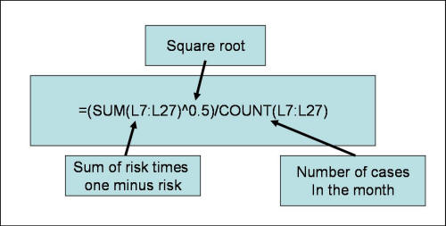
Figure 2:  Formula for Calculation of Expected Deviations from Table 1

Next you should have calculated the t-value.  Because there are different number of cases in each month, the t-value changes slightly.  The t-values were looked up in the table.  The relevant portion of the table is repeated here in Table 2.  Please note that t-values are assessed based on degrees of freedom which is equal to one minus the sample size. 

The control limits should be calculated from expected and not the observed rates.  This is a common mistake (look out for it).  To the expected rates we add or subtract the value of t times the standard deviation.  The UCL and LCL values I calculated were as follows:

Suggestions for Improvements

I hope this has been helpful feedback.