Risk-Adjusted Control Charts

Base on work of Eric L. Eisenstein, D.B.A.,¹ Charles F. Bethea, M.D. ²  Published in Health Care Management Science

From: ¹Duke University Medical Center, Durham, NC; ²Baptist Medical Center, Oklahoma City, OK

INTRODUCTION

Quality improvement professionals use control charts to examine whether changes in care processes has led to improvements in outcomes of care.  Historically control charts were first used in manufacturing.  Health care differs from manufacturing in that its primary input, patients, are not uniform [15,16]. Even within commonly performed procedures (e.g., CABG surgery or percutaneous coronary intervention), there are large differences in patient characteristics (i.e., patient mix) leading to different resource use [16, 22-25].   For this reason, control charts should be adjusted for patient characteristics (often referred to as risks).   Otherwise, lower acuity cases (with lower resource requirements) may be incorrectly identified as examples of excellent cost control while higher acuity cases (with higher resource requirements) may be incorrectly identified as examples of poor cost control. 

While risk-adjustment techniques have been developed for mortality [17-18, 27-28] and costs of care [23-25, 29], they are not generally applied in analysis of control charts. In fact, none of the leading books on analysis of control charts teach how risk adjustments should be made. 

Techniques for risk-adjusting p-charts have been developed [15]. Nonetheless, x-bar charts in health care continue to be presented without adequate risk-adjustment [14, 31]. In this paper we  begin by introducing techniques for risk-adjusting X-bar charts. We will then apply these techniques to the in-hospital care costs for CABG surgery (a common but expensive procedure) and will then compare differences between unadjusted and risk-adjusted X-bar chart results.

Our study population included all CABG surgery patients admitted to Baptist Medical Center, Oklahoma City, Oklahoma during the first ten months of fiscal year 1996. CABG surgery patients were defined as having an ICD-9-CM procedure code between 36.10 and 36.19. Patients with incomplete cost data and with concurrent percutaneous coronary intervention or valvular surgery procedures were excluded.

Clinical information used in our risk-adjustment model came from Baptist Medical Center’s implementation of the Duke Information System for Clinical Cardiology (DISCC). Both the DISCC system [32] and the risk-adjustment model used in this study [29] have been previously described. The patient characteristics selected for this model came from previous CABG surgery risk-adjustment models (cost and mortality) [23-24, 27-28] and from the expert opinion of clinical cardiologists and outcomes researchers at Baptist and Duke University Medical Centers.

All cost information used in our analyses came from Baptist Medical Center’s implementation of the Transition One cost accounting system. Transition One estimates hospital costs using a bottom-up approach that is based on resources consumed and their unit prices [33]. Our control chart analysis used the natural log of  in-hospital costs because CABG cost data is skewed to the right and must be transformed to meet the assumptions of Normal distribution [23, 34-35].

Methods For Developing Control Charts

Unadjusted Control Chart

The following formula detail the steps required to calculate lower and upper control limits for continuous variables in unadjusted X-bar control charts. Each time period is shown by the suffix "i", each patient is shown by the suffix "j".  Thus, X_ij is the observation for the jth patient in the ith time period.  Suffixes are dropped to designate an average; thus, X_i is the average of observations for all patients in time period "i", and X is the average for all patients in all time periods.  The number of cases in each time period is shown as n_i, the log costs of care for individual patient cases (x_ij), and the sum of log costs of care in time period "i" is shown as l_i.  The formulae for calculating the population average X, the population standard deviation S, average for time period "i" shown as X_i, standard deviation for time period "i" shown as S_i, upper control limits for time period "i" shown as UCL_i, and lower control limits for time period "i" shown as LCL_i are given below as equations (1) through (6).

An example of our calculations for the first month of our study (July) is shown below in equations (7) through (12). The degrees of freedom for the t-distribution are calculated as one less than the population sample size. The complete calculations for all study months are reported in Table 4 and the resulting unadjusted control chart is shown as Figure 1.

X = 5616.38  / 574                                       (7)

S = (55.49 / 573) ^0.5                          (8)

X₁= 474.21 / 49                         (9)

S₁= 0.31 / (49)^0.5                        (10)

UCL₁ = 9.7846 + (1.645 * 0.0445)            (11)

LCL₁ = 9.7846 - (1.645 * 0.0445)             (12)

Risk-Adjusted Control Chart

The following formulae detail the steps required to calculate lower and upper control limits for continuous variables in risk-adjusted X-bar control charts. The log of costs of care for case "j" in time period "i" is X_ij and the expected log of costs of care for case "j" in time period "i" is shown as E_ij.  The expected costs are predicted from the severity of the patient conditions using procedures described in citation [29].  The steps in calculating risk adjusted control limits are given in equations (13) through (17).

å _{j=1, …,m} E_ij /n_{i                                                 (13)}
D_ij = X_ij -E_ij                                            
D = å _{i=1, …nj  j=1, …,m} D_ij  /n                                    ₍₁₄₎
S = [å _{i=1, …nj  j=1, …,m} (D_ij –D)²/(n-1)] ^0.5                
S_i = S / (n_i =)^0.5                                                 (15)
UCL_i = E_i  + t * S_i                                             (16)
LCL_i = E_i  - t * S_i                                              (17)

An example of our calculations for the first month of our study (July) is shown below in equations (18) through (22). The degrees of freedom for the t-distribution are calculated as one less than the month’s sample size. The complete calculations for all study months are reported in Table 5 and the resulting unadjusted control chart is shown as Figure 2.

E₁ = 477.6779 / 49                (18)

d₁ = 3.4639 / 49                   (19)

S_d1 = 0.064 / (49) ^0.5                (20)

RESULTS

During the ten months of this study, in-hospital costs of CABG surgery at Baptist Medical Center averaged $18,859 (standard deviation $8,932, range $9604 to $126,830) and median costs were $16,773 (inter-quartile range $14,598 to $20,335). As anticipated, CABG surgery costs were skewed to the right with 73.9% of cases having costs less than $20,000, 20.4% having costs between $20,000 and $30,000, and 5.7% having costs > $30,000 (Figure 1).

Table 1: CABG Cost Distribution
Cost Range	Number of Cases	Percent of Cases
Less than $10,000	1	0.2
$10,000 - $19,999	423	73.7
$20,000 - $29,999	117	20.4
$30,000 - $39,999	23	4.0
$40,000 - $49,999	3	0.5
$50,000 - $59,999	0	0.0
$60,000 - $69,999	2	0.3
$70,000 - $79,999	4	0.7
$80,000	1	0.2

The number of cases per month ranged from 47 in March to 71 in September (Table 2). There was significant variation in average costs by month (range from $16,621 in July to $21,841 in February). However, there was less variation in average length of stay (range from 6.7 days in January to 8.4 days in February). In-hospital costs were correlated with the progression of months (July to April) (p = 0.017), whereas, length of stay was not (p = 0.796).

There also was significant monthly variation in the variables used in our CABG surgery risk-adjustment model (Table 3). Average age at admission varied in a rather tight band between 61.7 and 65.8 years. However, the percentage of patients with prior CABG surgery varied from 4.0% to 16.4% and patients with a history of congestive heart failure ranged from 1.6% to 18.0%. With regard to hospital process factors, the percentage of patients with acute myocardial infarction as the reason for admission ranged from 3.2% to 19.3% while those with an emergency admission ranged from 9.1% to 28.6%. Additionally, the percentage of patients with coronary angiography in the same admission as their CABG surgery procedure varied from 42.9% to 72.3%. Month of discharge independently explained 3.2% (p = 0.027) of the variation in log costs and our risk-adjustment model explained 32.0% (p = 0.001). However, month of discharge was not a significant predictor of log costs (p = 0.2044) after adjusting for differences in risk.

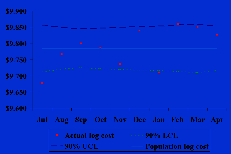
Unadjusted Control Chart

We used formulae (1) through (6) in calculating the unadjusted in-hospital CABG surgery costs by month (Table 4). These results are shown graphically in Figure 1.

The middle line in Figure 1 is the population’s average log costs for all ten months, the dashed lines are its 90% upper and lower confidence limits, and the small squares are the average log costs for each month. There is a trend toward increasing CABG costs over time in Figure 1 with the actual costs for three months (July, January, and February) being beyond the upper or lower control limit boundaries. Since only one month would be expected to be beyond these control limits by chance, this is an indication that the underlying CABG surgical process may be out of statistical control.

We used formulae (13) through (17) in calculating the risk-adjusted in-hospital CABG surgery costs by month (Table 5).

These results are shown graphically in Figure 2.

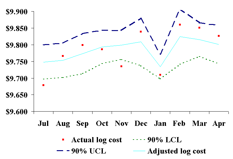
The middle line in Figure 2 is the risk-adjusted average log costs for each month, the dashed lines are its 90% upper and lower confidence limits, and the small squares are the average log costs for each month. After risk-adjustment, only two months (July and November) are beyond the upper or lower control limit boundary. Since only one month would be expected to be beyond these control limits by chance with a 90% confidence limit, there may be some cause for concern. Additionally, two of the months whose average CABG surgery costs were beyond the 90% control limit boundary without risk-adjustment (January and February) are now within these limits and may be instances of wider risk variation rather than cost outliers.

As financial pressures continue to increase in the US health care environment, hospitals will continue to investigate ways to control their costs of care. Because CQI techniques have been successfully applied in the manufacturing sector of the US economy, there has been great hope that they can achieve equivalent success in managing the ever escalating costs within the health care sector. Unfortunately, health care has an additional source of variation (patient mix) which has not typically been included in health care control charts. Our study demonstrates the value of risk-adjustment when developing control charts for health care. Without risk-adjustment, three of the months we studied had average costs beyond the lower or upper control limit boundaries and there appeared to be a trend toward higher (and potentially out of statistical control) costs. After risk-adjustment, only two months had average costs beyond their control limit boundaries and our trend toward higher costs over time was seen as a trend to increasing patient acuity, which is associated with higher expected health care costs.

Although the value of risk-adjustment in control charts has not been previously demonstrated, there is evidence that it could be beneficial when studying CABG surgery outcomes. Previous studies have demonstrated the value of risk-adjustment when making comparisons among surgeons, hospitals, and payers [23, 24, 29]. Thus, we can assume that risk-adjustment techniques would be beneficial in other types of analysis in which continuous outcome variables may be expected to vary based upon differences in baseline patient characteristics.

While the methods used in our analyses are simple, our information requirements may be beyond those available to many community hospitals. Our analyses require information from a surgical information system to construct a risk-adjustment model as well as information from a hospital-wide cost accounting system to measure total in-hospital costs. Additionally, our methods may not be feasible for other types of procedures which have lower average costs of care or which occur less frequently.

Although log transformation is required when cost data is highly skewed to the right, the resulting data is extremely difficult to present to health care administrators. We experimented with smearing as a method for retransforming the data [36]. The retransformed data was more understandable, but its spread was greater than the logged data and incorrectly produced a greater number of months with average cost beyond the upper and lower control limit boundaries. Since the log transformed and retransformed data did not identify the same outliers, we would not recommend smearing as a means for retransforming data for control charts.

Sample size is an obvious limitation of our analysis. If we had more months and more cases per month, our results would have been more compelling. Nonetheless, ten months of data did demonstrate the value of risk-adjustment in control charts. We are currently analyzing three years of CABG surgery data from Baptist Medical Center and hope to present these results in the near future.

Although risk-adjustment may not be required for all health care control charts, it proved valuable in the present analysis by allowing us to adjust our results for monthly differences in patient mix. risk-adjustment demonstrated that the trend we saw in CABG costs paralleled the increasing acuity in CABG patients. Thus, the higher costs in succeeding months were the result of increasing patient acuity and not the result of a surgical process which was potentially out of control.

1. T.L. Adams, Physicians and administrators may be ready to embrace profiling. Healthcare Financial Management 52 (1998) 94.
2. J.E. Evans III, Y. Hwang, N. Nagarajan, Physicians’ response to length-of-stay profiling. Medical Care 33 (1995) 1106 - 1111.
3. M.R. Gold, R. Hurley, T. Lake, T. Ensor, R. Berenson, A national survey of the arrangements managed-care plans make with physicians. New England Journal of Medicine 25 (1995) 1678 - 83.
4. Health Care Financial Management Association, Financial and clinical benchmarking: The strategic use of data. HCIA and The Health Care Financial Management Association 1997.
5. E.J. Sessa, Public disclosure: A response from the Pennsylvania Health Care Cost Containment Council experience, in: Physician Profiling and Risk Adjustment, ed. N. Goldfield, (Aspen Publishers, Gaithersburg, MD, 1995) 111 - 6.
6. N.J. Banks, R.H. Palmer, D.M. Berwick, and P. Plsek, Variability in clinical systems: applying modern quality control methods to health care, Joint Commission Journal on Quality Improvement 21 (1995) 407 - 19.
7. D.M. Berwick, Continuous improvement as an ideal in health care, New England Journal of Medicine 320 (1989) 53 - 6.
8. D. M. Berwick, Controlling variation in health care: a consultation from Walter Shewhart, Medical Care 29 (1991) 1212 - 25.
9. D. Blumenthal and A.C. Scheck, Improving Clinical Practice: Total Quality Management & The Physician, (Jossey-Bass Publishers, San Francisco, 1995)
10. W. E. Deming, The New Economics: For Industry, Government, Education, 2^nd Edition, (Massachusetts Institute of Technology Center for Advanced Educational Services, Cambridge, 1997).
11. C.M. Kilo, A. Kabcenell, and D.M. Berwick, Beyond survival: toward continuous improvement in medical care, New Horizons 6 (1998) 3 - 11.
12. G. Laffel, D. Blumenthal, The case for using industrial quality management science in health care organizations, Journal of the American Medical Association 262 (1989) 2869 - 73.
13. S.M. Shortell, R.R. Gillies, D.A. Anderson, K.M. Erickson, J.B. Mitchell, Remaking health care in America: building organized delivery systems, (Jossey-Bass Inc, San Franciso, 1996).
14. R.B. Fetter, DRGs and quality management in hospitals, in: Physician Profiling and Risk Adjustment, ed. N. Goldfield, (Aspen Publishers, Gaithersburg, MD, 1995) 171-188.
15. F. Alemi, W. Rom, and E.L. Eisenstein, Risk-adjusted control charts, Annals of Operations Research 67 (1996) 45 - 60.
16. E.L. Eisenstein and J.W. Hales, A clinical economics workstation for risk-adjusted health care cost management, Proceedings - the Annual Symposium on Computer Applications in Medical Care (1995) 620 - 4.
17. L.I. Iezzoni, Risk Adjustment for Measuring Healthcare Outcomes 2^nd Edition (Health Administration Press, Chicago, 1997).
18. N. Goldfield, Physician Profiling and Risk Adjustment 2^nd Edition (Aspen Publishers, Gaithersburg, 1999).
19. E. Braunwald, R.H. Jones, D.B. Mark, J. Brown, L. Brown, M.D. Cheitlin, C.A. Concannon, M. Cowan, C. Edwards, V. Fuster V, Diagnosing and managing unstable angina. Agency for Health Care Policy and Research. Circulation 90 (1994) 613 - 22.
20. H.V. Anderson, C.P. Cannon, P.H. Stone, D.O. Williams, C.H. McCabe, G.L. Knatterud, B.Thompson, J.T. Willerson, E. Braunwald, One-year results of the Thrombolysis in Myocardial Infarction (TIMI) IIIB clinical trial. A randomized comparison of tissue-type plasminogen activator versus placebo and early invasive versus early conservative strategies in unstable angina and non-Q wave myocardial infarction. Journal of the American College of Cardiology 26 (1995) 1643 - 50.
21. G.W. Barsness, E.D. Peterson, E.M. Ohman, C.L. Nelson, E.R. DeLong, J.G. Reves, P.K. Smith, R.D. Anderson, R.H. Jones, R.M. Califf, Relationship between diabetes mellitus and long-term survival after coronary bypass and angioplasty. Circulation 96 (1997) 2551 - 6.
22. E.L. Eisenstein, Patient risk or physician practice: What factors drive costs in unstable angina? American Heart Journal 136 (1998) 365 - 7.
23. L.R. Smith, C.A. Milano, B.S. Molter, J.R. Elbeery, D.C. Sabiston Jr.and P.K. Smith, Preoperative determinants of postoperative costs associated with coronary artery bypass graft surgery, Circulation 90 (1994) II124 - 8.
24. P.A. Cowper, E.R. DeLong, E.D. Peterson, J. Lipscomb, L.H. Muhlbaier, J.G. Jollis, D.B. Pryor and D.B. Mark, Geographic variation in resource use for coronary artery bypass surgery. IHD Port Investigators, Medical Care 35 (1997) 320 - 333.
25. E.D. Peterson, P. A. Cowper, E. R. DeLong, J. P. Zidar, R. S. Stack, D. B. Mark, Acute and long-term cost implications of coronary stenting. Journal of the American College of Cardiology 33 (1999) 1610 - 1618.
26. S. Greenfield, Continuous Quality Improvement and the Physician: Building Bridges with Outcomes Research, in: Improving Clinical Practice: Total Quality Management & The Physician, ed. D. Blumenthal, (Jossey-Bass Publishers, San Francisco, 1995).
27. E.L. Hannan, H. Kilburn Jr., M. Racz, E. Shields and M.R. Chassin, Improving the outcomes of coronary artery bypass surgery in New York State, Journal of the American Medical Association 271, (1994) 761 - 6.
28. E.R. DeLong, E.D. Peterson, D.M. DeLong, L.H. Muhlbaier, S. Hackett and D.B. Mark, Comparing risk-adjustment methods for provider profiling, Statistics in Medicine 16 (1997) 2645 - 64.
29. E.L. Eisenstein, L.H. Muhlbaier, C.F. Bethea, E.D. Peterson, W.H. Oehlert, J.A. Stafford and D.B. Mark, The importance of payer case mix on hospital costs: Don’t contract without it, Journal of the American College of Cardiology 33 (1999) 248A.
30. D. Neuhauser, L. Headrick, W. Katcher and P. Lucas, Applying the Statistical Methods of Continuous Quality Improvement to Primary Care: Hypertension, in: Improving Clinical Practice: Total Quality Management & The Physician, ed. D. Blumenthal, (Jossey-Bass Publishers, San Francisco, 1995).
31. F.C. Kaminsky, J. Maleyeff and D.L. Mullins, Using SPC to analyze measurements in a healthcare organization, Journal of Healthcare Risk Management Winter (1998) 36 - 46.
32. D.B. Mark, C.L. Nelson, R.M. Califf, F.E. Harrell Jr, K.L. Lee, R.H. Jones, D.F. Fortin, R.S. Stack, D.D. Glower and L.R. Smith, Continuing evolution of therapy for coronary artery disease: initial results from the era of coronary angioplasty, Circulation 89 (1994) 2015 - 2025.
33. E.L. Eisenstein and D.B. Mark, Economic Issues Related to Diagnosis and Therapy for Coronary Heart Disease, in Diagnostic and Therapeutic Cardiac Catheterization, 3^rd edition, ed. C.J. Pepine (Williams & Wilkins, Baltimore,1998) 892-913.
34. X-H. Zhou, C.A. Melfi, S.L. Hui, Methods for comparison of cost data, Annals of Internal Medicine 127 (1997) 752 - 756.
35. J. Lipscomb, M. Ancukiewicz, G. Parmigiani, V. Hasselblad, G. Samsa and D.B. Matchar, Predicting the cost of illness: a comparison of alternative models, Medical Decision Making 18 (1998) S39 - S56.
36. N. Duan, Smearing estimate: a nonparametric retransformaton method, Journal of the American Statistical Association 78 (1983) 605 - 610.