|
|
 |
|||||||||||||||||||||||||||||||||||||||||||||||||||||||||||||||||||||||||||||||||||||||||||||||||||||||||||||||||||||||||||||||||||||||||||||||||||||||||||||||||||||||||||||||||||||||||||||||||||||||||||||||||||||||||||||||||||||||||||||||||||||||||||||||||||||||
Measuring UncertaintyThis section describes how probability can quantify how uncertain we feel about future events. We describe:
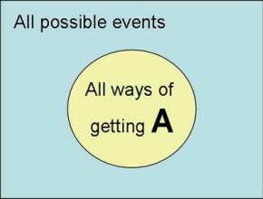
Measuring uncertainty is important because it allows us to make tradeoffs among uncertain events. It allows us to act in uncertain environments. We may not be sure about a business outcome, but if we knew the chances were good for it occurring, we may pursue it. What is Probability?When we are sure that an event will occur, we say that it has a probability of 1. When we are sure that an event will not occur, we assign it a probability of zero. When we are completely in dark, we give it a probability of 0.5, a fifty - fifty chance of occurrence. All other values between 0 and 1 measure how uncertain we are about the occurrence of the event. The best way to think of probabilities is as the ratio of all ways in which an event may occur divided by all possible events. In short, probability is the prevalence of the event among the possible events. The probability of a small business failing is then the number of business failures divided by the number of small businesses. The probability of an iatrogenic infection in the last month in our hospital is the number of patients who last month had an iatrogenic infection in our hospital divided by the number of patients in our hospital during last month. Graphically, we can show a probability by defining the square to be proportional to the number of possible events and the circle as the all ways in which event A occurs; then the ratio of the circle to the square is the probability of A (see Figure 1).
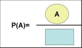
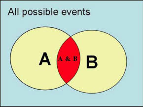
Figure 1: A Graphical Intuition for Definition of Probability The rules of probability allow us to calculate probability of combination of events using the above definition of probabilities. The probability of two events A and B occurring together, is calculated by first summing all the possible ways in which event A will occur plus all the ways in which event B will occur, minus all the possible ways in which both event A and B will occur (this term is subcontracted because it is double counted). This sum is divided by the all possible ways that any event will occur. This is represented in mathematical terms as: P(A or B) = P(A) + P(B) - P(A & B) Graphically, the concept can be shown as the yellow and red areas in Figure 2 divided by the blue area.
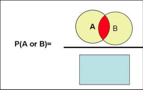
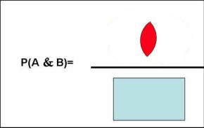
Figure 2: Graphical Representation of Probability of A or B Similarly, the probability of A and B occurring together, corresponds to the overlap between A and B and can be shown graphically as the red area divided by all possible events (the rectangular blue area) in Figure 3.
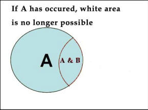
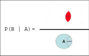
Figure 3: Graphical Representation of Probability A and B The definition of probability gives us a simple calculus for combining uncertainty of two events. We can now ask questions such as: "What is the probability that frail elderly (age>75) or infants will join our HMO?" According to our formulas this can be calculated as: P( Frail elderly or Infants join HMO) = Since the chance of being frail elderly and infant is zero (i.e. the two events are mutually exclusive), we can re-write the formula as: P( Frail elderly or Infants join HMO) = P( Frail elderly join HMO) + P( Infants join HMO) The definition of probability also helps us calculate the probability of an event conditioned on the occurrence of other events. In these circumstances, we know something has happened and we are asking for the calculation of the probability of another event. In mathematical terms we show this as P(A | B) and read it as probability of A given B. When an event occurs, it reduces the remaining list of possibilities; we no longer need to track the possibility that the event may not occur. We can use our definition of probabilities to calculate conditional probabilities by restricting the possibilities to only events that we know have occurred. Graphically, this is shown as in Figure 4.
Figure 4: Probability of B Given A is Calculated by Reducing Possibilities For example, we can now calculate the probability that a frail elderly joins the HMO and is hospitalized. Instead of looking at hospitalization rate among frail elderly, we need to restrict the possibilities to frail elderly who have join the HMO. Then the probability is calculated as the ratio of hospitalization among frail elderly in the HMO to number of frail elderly in the HMO. For another example, consider that an analysis has produced the following joint probabilities for the patient being in treatment or in probation:
Please note that table 1 provides joint and marginal probabilities by dividing the observed frequency of days by the total number of days examined. Marginal probabilities refer to the probability of one event. In Table 1 these are provided in row and column named "total." Joint probability refers to the probability of two events co-occurring at same time. In Table 1, these are provided in the cell values not labeled as "Total." For example, the joint probability of having both probation and treatment day is 0.51. This probability is calculated by dividing the number of days in which both probation and treatment occur by the total number of days examined. The total number of days is referred to as the universe of possible days. If the analyst wishes to calculate a conditional probability, the total universe of possible days must be reduced to days with the condition. Suppose the analyst wants to calculate the conditional probability of being in treatment given that the patient is already in probation. In this case, the universe is reduced to all days in which the patient was in probation. In this reduced universe, the total number days of treatment is the number of days of having both treatment and probation. Therefore, the conditional probability of treatment given probation is: p(Treatment day | Probation day) = Since Table 1 provides the joint and marginal probabilities, we can describe the above calculations in terms of joint and marginal probabilities by dividing the top and bottom of the above division by the total number of possible days: p(Treatment day | Probation day) = P(Both treatment and probation) / p(Probation) p(Treatment day | Probation day) = 0.51/0.56 = 0.93 The point of this example is that conditional probabilities can be calculated easily by reducing the universe examined to the condition. You can calculate conditional probabilities from marginal and joint probabilities if you keep in mind how the condition has reduced the universe of possibility. Conditional probabilities are a very useful concept. They allow us to think through an uncertain sequence of events. If each event can be conditioned on its predecessor, a chain of events can be examined. Then if one component of the chain changes, we can calculate the impact of the change through out the chain. In this sense, conditional probabilities show how a series of clues might forecast a future event. The point of this introduction has been that the calculus of probability is an easy way to track the overall uncertainty of several events. The calculus is appropriate if several simple assumptions are me. These include the following:
If a set of numbers assigned to uncertain events meet these three principles, then it is a probability function and the numbers must follows the algebra of probabilities. Odds & ProbabilitySome people prefer to describe their uncertainty about an event in terms of odds for the event occurring and not use the concept of probability. The two concepts are related. Odds are expressed as ratios while probabilities are expressed as decimals between 0 and 1. The odds for an event is related to its probability by the following formula: Odds of an event = Probability of the event / (1-Probability of the event) Probability of an event = Odds of the event / (1+Odds of the event) For example, if the probability of an event is 90%, the odds for it is 0.9/(1-0.9) = 9 to one. If the odds of an event is 2 to one, the probability for the event is 2/(1+2) = .66. Odds and probabilities are always positive numbers. There is no upper limit to an odd ratio but the maximum probability is 1. An odds of 1 to 1, implies a 50% chance or a probability of 0.50. This shows that the person is completely uncertain about the event. Odds of 2 to 1 increase the probability of the event to 0.66. Odds of 3 to 1 increases the probability of the event to 0.75 and odds of 4 to 1 increases the probability of the event to 0.8. Sources of DataThere are two ways to measure probability of an event.
Both methods produce probabilities, but one approach is objective and the other is based on opinions. Both approaches measure the degree of uncertainty about the success of the HMO, but there is a major difference between them. Objective frequencies are based on observation of the history of the event, while measurement of strength of belief is based on an individual's opinion, even about events that have no history (e.g. what is the chance that there will be a terrorist attack in our hospital). Savage (1954) and DeFinetti (1964) argued that the rules of probabilities can work with uncertainties expressed as strength of opinion. Savage termed the strength of a decision maker's convictions "subjective probability" and used the calculus of probability to analyze them. Subjective probability can be measured along two different concepts: (1) intensity of feelings and (2) hypothetical action (Ramsey 1950). We measure subjective probability on the basis of intensity of feelings by asking an expert to mark a scale between 0 and 1. We measure subjective probability on the basis of hypothetical actions by asking the expert about the hypothetical frequency that the event will occur. Suppose we want to measure the probability that an employee will join the HMO. Using the first method, we would ask an expert on the local health care market about intensity of feeling:
When measuring according to hypothetical frequencies, we ask the expert to imagine what frequency he or she expects. While the event has not occurred repeatedly, we can ask the expert to imagine that it has.
Can one apply the calculus of probability to analyze frequency counts to analyze subjective probabilities? If both the subjective and the objective methods produce a probability for the event, then obviously the calculus of probabilities can be used to make new inferences from these data. When strength of belief is measured as a hypothetical frequency, we can easily show that beliefs can be treated as probability functions. Note that we are not saying that they are but that they should. If the frequency is observed or described by an expert, it makes no difference; the resulting number should follow the rules of probability. But how can we argue that subjective probabilities measured as intensity of feelings should be treated as probability functions? To answer this, we must return to the formal definition of a probability measure. A probability function was defined by the following characteristics:
These assumptions are at the root of all mathematical work in probability, so any beliefs expressed as probability must follow them. Furthermore, if these three assumptions are met, then the numbers produced in this fashion will follow all rules of probabilities. Are these three assumptions met? The first assumption is always true, because we can assign numbers to beliefs so they are always positive. But the second and third assumptions are not always true, and people do hold beliefs that violate them. We can, however, take steps to ensure that these two assumptions are also met. For example, when the estimates of all possibilities (e.g., probability of success and failure) do not total 1, we can standardize the estimates to do so. When the estimated probabilities of two mutually exclusive events do not equal the sum of their probabilities, we can ask whether they should, and adjust as necessary. In their thinking, decision makers may or may not follow the calculus of probability. But what people do and how they should do it are two different issues. Decision makers may wish to follow the rules of probability, even though they have not always done so. Experts' opinions may not follow the rules of probability but if experts agree with the three principles listed above, then such opinions should follow the rules of probability. Our argument is not that probabilities and beliefs are the identical constructs, but rather that probabilities provide a context in which beliefs can be studied. That is, if beliefs are expressed as probabilities, the rules of probability provide a systematic and orderly method of examining the implications of these beliefs. Bayes FormulaFrom definition of conditional probability, one can derive the Bayes formula. It an optimal model for revising existing opinion (sometimes called prior opinion) in the light of new evidence or clues. The theorem states:
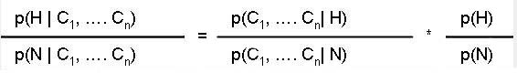
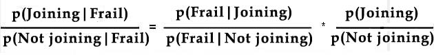
In words, Bayes theorem states: Posterior odds after review of clues = Likelihood ratio associated with the clues * Prior odds The difference between the left and right turn is the knowledge of clues. Thus, the theorem shows how our opinion about the hypothesis should change after examining clues 1 through n. Because Bayes' theorem prescribes how opinions should be revised to reflect new data, it is a tool for consistent and systematic processing of opinions. We are claiming that prior odds of an event is multiplied by the likelihood ratio associated with various clues to obtain the posterior odds for the event. At first glance this may seem odd. You may ask why multiply, why not add? Why not include some other probabilities besides prior odds and likelihood ratios? Let us make the case why Bayes formula is logical and should make sense to you. We are not trying to prove the formula but to appeal to your intuitions and show you that it fits your expectations about how opinions should be revised. Bayes' theorem was first proven mathematically Thomas Bayes, an English mathematician, although he never submitted his paper for publication. Using Bayes' notes, Price presented a proof of Bayes' theorem. The following presentation of Bayes' argument differs from the original (Bayes 1963). We will consider for the sake of argument that there is only one characteristic of interest, say familiarity with computers. If we knew who will join and who will not, we could establish four groups:
Let us suppose the HMO is offered to "a + b + c + d" Medicare beneficiaries (see Table 2). We define probability of an event as the number of ways the event occurs divided by the total possibilities. Thus, since the total number of beneficiaries is a + b + c + d; then the probability of any of them joining the program is the number of people who join divided by the total number of beneficiaries: P( Joining) = (a +.b) / (a + b + c + d) Similarly, the chance of finding a frail elderly, P(frail elderly), is the total number of frail elderly, a + c, divided by the total number of beneficiaries: P( Frail) = (a + c) / (a + b + c + d) Now consider a special situation, where we focus only on those beneficiaries that are frail. Given that our focus is on this subset, now the total number of possibilities is reduced from the total number of beneficiaries to the the number frail, i.e. a +c. If we focus only on the frail elderly, the probability of one of these beneficiaries joining is given by P( Joining I Frail) = a / (a + c) And similarly, the likelihood that we will find frail elderly among joiners is given by reducing the total possibilities to only those beneficiaries that join the HMO and counting how many were frail elderly: P( Frail | Joining) = a / (a + b) Using the above four formulas, we see that: P( Joining I Frail) = P( Frail | Joining) * P( Joining) / P( Frail) Repeating the procedure for not joining the HMO we find: P( Not joining I Frail) = P( Frail | Not joining) * P( Not joining) / P( Frail) Dividing the above two equations we get the the odds form of the Bayes formula:
As the above has shown, the Bayes formula follows from very reasonable assumptions about the beneficiaries. The point is that if we partition beneficiaries into the four groups, count the number in each group, and define probability of an event as the count of the event divided by number of possibilities, then Bayes' formula follows. Most readers will agree that the assumptions we have made are reasonable and therefore the implication of these assumptions, i.e. the Bayes formula, should also be reasonable. IndependenceIn probabilities, the concept of independence has a very specific meaning. If two events are independent of each other, then the occurrence of one event does not tell us much about the occurrence of the other event. Mathematically, this condition can be presented as: P(A | B) = P(A) Independence means that the presence of one clue does not change the value of another clue. An example might be prevalence of diabetes and car accidents; knowing the probability of car accidents in a population will not tell us anything about the probability of diabetes. When two events are independent, we can calculate the probability of both co-occurring from the marginal probabilities of each event occurring: P(A&B) = P(A) * P(B) Thus we can calculate the probability of a diabetic having a car accident as the product of the probability of being diabetic and probability of a car accident. A related concept, is conditional independence. Conditional independence means that for a specific population, presence of one clue does not change the probability of another. Mathematically, this is shown as: P(A | B, C) = P(A | C) The above formula reads that if we know that C has occurred, telling us that B has occurred does not add any new information to the estimate of probability of event A. Another way of saying this is to say that in population C, knowing B does not tell us much about chance for A. As before, conditional independence allows us to calculate joint probabilities from marginal probabilities: P(A&B | C) = P(A | C) * P(B | C) The above formulas says that among the population C, the probability of A & B occurring is equal to the product of probability of each event occurring. It is possible for two events to be dependent, but when conditioned on the occurrence of a third event they may become independent of each other. For example, we may think that scheduling long shifts will lead to medication errors. Thus we may show (≠ means not equal to): P( Medication error ) ≠ P( Medication error| Long shift) At the same time, we may consider that in the population of employees that are not fatigued (even though they have long shifts), the two events are independent of each other, i.e. P( Medication error | Long shift, Not fatigued) = P( Medication error| Not fatigued) This example shows that related events may become independent under certain condition. Independence and conditional Independence are invoked often to simplify calculation of complex likelihoods involving multiple events. We have already shown how independence facilitates the calculation of joint probabilities. The advantage of verifying independence becomes even more pronounced when examining more that two events. Recall that the use of Bayes Odds form requires the estimation of the likelihood ratio. When multiple events are considered before revising the prior odds, the estimation of the likelihood ratio involves conditioning future events on all prior events:
P(C1,C2,C3,
...,Cn|H1)
= P(C1|H1)
* P(C2|H1,C1)
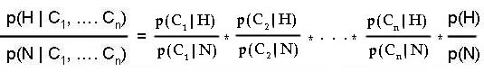
* Note that each term in the above formula is conditioned on previous events. When events are considered, the posterior odds is modified and in addition they are used to condition all subsequent events. Note that all terms are conditioned on the hypothesis. The first term is conditioned on no additional event; the second term is conditioned on the first event; the third term is conditioned on the first and second event and so on until the last term that is conditioned on all subsequent n-1 events. If we stay with our analogy that conditioning is reducing the sample size to the portion of the sample that has the condition, then the above formula suggests a sequence for reducing the sample size. Because there are many events, the data has to be portioned in increasingly smaller size. Obviously, for data to be partitioned so many times, one needs a large database. Conditional independence allows us to calculate likelihood ratios associated with a series of events without needing large databases. Instead of conditioning the event on the hypothesis and all prior events, we can now ignore all prior events: P(C1,C2,C3, ...,Cn | H) = P(C1 | H) * P(C2 | H) * P(C3 | H) * P(C4 | H) * ... * P(Cn | H) Conditional independence simplifies the calculation of the likelihood ratios. Now we can re-write Bayes odds form in terms of the likelihood ratio associated with each event.
In words the above formula states:
The above formulas has many applications. It is often used to estimate how various clues (events) may help revise prior probability of a target event. For example, we might use the above formula to predict the posterior odds of hospitalization for a frail elderly female patient, if we accept that age and gender are conditionally independent of each other. Suppose the likelihood ratio associated with frail elderly is 5/2, meaning that knowing the patient is frail elderly will increase the odds of hospitalization by 2.5 times. Also suppose that knowing the patient is female reduces the odds for hospitalization by 9/10. Now, if the prior odds for hospitalization is 1/2, the posterior odds for hospitalization can be calculated using the following formula:
The posterior odds of hospitalization can now be calculated as:
For mutually exclusive and exhaustive events, odds for an event can be turned into probability of the event by using the following formula: Probability = Odds /(1+Odds) Using the above formula, we can calculate the probability of hospitalization as: Probability of hospitalization = 1.125 /(1+1.125) = 0.53 Verifying IndependenceThere are several ways to verify conditional independence. These include (1) reducing sample size, (2) correlations, (3) direct query from experts and (4) separation in causal maps. (1) Reducing sample sizeIf data exist, conditional independence can be verified by selecting the population that has the condition and verifying that the product of marginal probabilities is equal joint probability of the two events. For example, in Table 3, eighteen cases from a special unit prone to medication errors are presented. The question is whether rate of medication errors is independent of length of work shift.
Using the data in Table 3, the probability of medication error is calculated as: P( Error) =
Number of cases with errors / Number of cases = 6/18 = 0.33 Above calculations show that probability of medication error and length of shift are not independent of each other. Knowing the length of the shift tells us something about the probability of error in that shift. But consider the situation where we are examining these two events among cases where the provider was fatigued. Now the population of cases we are examining is reduced to the cases 1 through 8. With this population, calculation of the probabilities yields: P( Error |
Fatigued) = 0.50 P( Error & Long shift |
Fatigued) = 0.25
Among fatigued providers, medication error is independent of length of work shift. The procedures used in this example, namely calculating the joint probability and examining to see if it is approximately equal to product of the marginal is one way of verifying independence. Independence can also be examined by calculating conditional probabilities. As before conditional probabilities are calculated by restricting the population size. For example, in the population of fatigued providers (i.e. in cases 1 through 8) there are several cases of working in long shift (i.e. in cases 1, 2, 5, and 8). We can use this information to calculate conditional probabilities: P( Error | Fatigue) = 0.50 Again we observe that among fatigued workers knowing that the work shift was long adds no information to the probability of medication error. The above procedures shows how independence can be verified by counting cases in reduced populations. In case there is considerable amount of data available inside a database, the approach can easily be implemented by using Standard Query Language. To calculate the conditional probability of an event, all we need to do is to run a select query that would select the condition and count the number of events of interest. (2) Correlation analysisOne way for verifying independence so is to examine the correlations. Two events that are correlated are dependent. For example in Table 4, we can examine the relationship between age and blood pressure by calculating the correlation between these two variables.
Table 4: Relationship between Age and Blood Pressure in 7 Patients The correlation between the age and blood pressure, in the sample of data in Table 4, is 0.91. This correlation is relatively high and suggests that knowing something about the age of the person will tell us a great deal about the blood pressure. Therefore, age and blood pressure are dependent in our sample. Correlations can also be used to verify conditional independence. To examine independence of event A and B, in population where event C has occurred, we need to introduce three pair wise correlations. Assume:
Events A and B are conditionally independent of each other if the "Vanishing Partial Correlation" condition holds. This condition states: Rab= Rac Rcb Using the data in Table 4, we calculate the following correlations:
Examination of the data shows that the vanishing partial correlation holds (~ means approximate equality): Rage, blood pressure = 0.91 ~ 0.82 * 0.95 = Rage, weight * R weight, blood pressure Therefore, we can conclude that given the patients' weight, the variables age and blood pressure are independent of each other because they have a partial correlation of zero. (3) Directly ask expertsIt is not always possible to gather data. Sometimes independence must be verified subjectively by asking about the relationship among the variables from a knowledgeable expert. Unconditional independence can be verified by asking the expert to tell if knowledge of one event will tell us a lot about the likelihood of another. Conditional independence can be verified by repeating the same task but now within specific populations. Gustafson and others (1973a) described a procedure for assessing independence by directly querying experts:
Experts will have in mind different, sometimes wrong, notions of dependence, so the words conditional dependence should be avoided. Instead, we focus on whether one clue tells us a lot about the influence of another clue in specific populations. We find that experts are more likely to understand this line of questioning as opposed to directly asking them to verify conditional independence. (4) Separation in causal mapsOne can assess dependencies through analyzing maps of causal relationships. In a causal network each node describes an event. The directed arcs between the nodes depict how one event causes another. Causal networks work for situations here there is no cyclical relationship among the variables; it is not possible to start from a node and follow the arcs and return to the same node. An expert is asked to draw a causal network of the events. If the expert can do so, then conditional dependence can be verified by the position of nodes and the arcs. Several rules can be used to identify conditional dependencies in a causal network (Pearl, 1998, p117). These rules include the following:
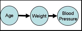
In the above rules, we assume that removing the condition will actually remove the path between the independent events. "If removal of node C renders nodes A and B disconnected from each other, then A and B are proclaimed independent from each other given C. Another way to say this is to observe that event C is between events A and B and there is no way of following the arcs from A to B without passing through C. In this situation, P(A | B,C) = P(A | C), A is independent of B given C. For example, an expert may provide the map in Figure 5 for the relationships between age, weight and blood pressure.
Figure 5: A Causal Map for Relationship of Age and Blood Pressure In this Figure, age and weight are shown to depend on each other. Age and blood pressure are show to be conditionally independent of each other because there is no way of going from one to the other without passing through the weight node. Note that if there was an arc between age and blood pressure, i.e. if the expert believed that there was a direct relationship between these two variables, then conditional independence would be violated. Analysis of causal maps can help identify a large number of independencies among the events being considered. We will present more details and examples for using causal models to verify independence when we discuss root cause analysis and modeling uncertainty in subsequent chapters. Time to EventA method that can allow us to examine rare events directly is through examination of time to the event. If we assume that an event has a Bernoulli distribution (i.e. the event either happens or does not happen, it has a constant probability of occurrence, and the probability of the event does not depend on prior occurrences of the event); then number of consecutive occurrences of the event has a Geometric distribution. In a geometric distribution, probability of a rare event, p, can be estimated from the average time to the event, t, using the following formula: p = 1 / (1+t) Table 1 shows how this relationship can be explored to calculate rare probabilities. The expert is asked to provide the dates for the last few times the event has occurred in the last year or decade. The average time to reoccurrence is calculated and the above formula is used to estimate the probability of the event.
For example, suppose we want to know what is the probability of an a terrorist attack in city of Washington DC. To calculate this probability, we need only to record the dates of the last attacks in the city and average the time between the attacks. This average time between the reoccurrence of the event can then be used to estimate the probability of another attack. For another example, suppose we do not know the frequency of medication errors in our hospital. Furthermore, suppose that last year there were two reports of medication errors, one at start of the year and one in the middle of the year. The pattern of medication error suggests 6 months time between errors. Average time between errors allows us to estimate the daily probability of medication error: P( Error) = 1 / (1+6*30) = 0.0056 What Do You Know?Advanced learners like you, often need different ways of understanding a topic. Reading is just one way of understanding. Another way is through writing. When you write you not only recall what you have written but also may need to make inferences about what you have read. Please complete the following assessment: Presentations
To assist you in reviewing the material in this lecture, please see the following resources:
Narrated lectures require use of Flash. More
Copyright © 1996 Farrokh Alemi, Ph.D. Created on Tuesday, September 17, 1996. Sunday, October 06, 1996 4:20:30 PM Most recent revision 01/15/2019. This page is part of a course lecture on Measuring Uncertainty |
|||||||||||||||||||||||||||||||||||||||||||||||||||||||||||||||||||||||||||||||||||||||||||||||||||||||||||||||||||||||||||||||||||||||||||||||||||||||||||||||||||||||||||||||||||||||||||||||||||||||||||||||||||||||||||||||||||||||||||||||||||||||||||||||||||||||
|
|
|||||||||||||||||||||||||||||||||||||||||||||||||||||||||||||||||||||||||||||||||||||||||||||||||||||||||||||||||||||||||||||||||||||||||||||||||||||||||||||||||||||||||||||||||||||||||||||||||||||||||||||||||||||||||||||||||||||||||||||||||||||||||||||||||||||||