HAP 525: 

Risk Analysis in Healthcare

Self Experiments and Analytical Relapse Prevention

Introduction

When clients want to change, occasionally they fail and relapse to old habits.  In these circumstances, it is important to understand causes of relapse so that clients can address the root cause of the problem.  Often clients focus on their motivation and not on the events and routines that lead to the relapse.  As a result, relapses reoccur and clients fail to maintain their new habits.  This page is organized to improve understanding of root causes of relapse into poor habits.

Clinicians are encouraged to ask if clients have exercised sufficiently, reduced excess weight, stopped abuse of substances, or failed to comply with clinician's advice in any manner.  The real question, of course, is not whether they have but why.  Unfortunately, neither the clinician nor the client may know why they behave the way they do.  At some superficial level, everyone can have an excuse.  But further investigation may reveal root causes that are surprisingly hidden and seemingly unrelated to the behavior.  A client may fail to exercise because of a side effect of a medication they are taking, poor sleep routines, rain, and many other reasons.  Neither the clinician or the client may know the root cause of their behavior.  The purpose of analytical relapse prevention is to reveal the root causes of behavior so that clinicians and clients can aggressively change these root causes. 

Relapse prevention is widely practiced in substance abuse treatment (Jaffe, 2002; Larimer, Palmer, Marlatt 2005; Kadden 1996; McKay 1999). Clients are asked to retrospectively review their habits and examine what leads to their return to drug use.  Unfortunately, current relapse prevention efforts accepts the client's claim of cause and effect as valid.  The literature shows that human beings are notoriously poor in correct attributions of causes of events (Cherpitel, Bond, Ye, Borges, Room, Poznyak, Hao, 2006; Billing, Bar-On, Rehnqvist 1997; Ladd, Welsh, Vitulli, Labbe, Law 1997).  The most notorious fallacy in causal attribution is that success is due to my skills and failures are due to event outside of client's control (Ahn, Kalish, Medin, Gelman 1995; Green, Bailey, Zinser, Williams 1994; Kinderman, Kaney, Morley, Bentall 1992).  In analytical relapse prevention mathematical tools are used to identify root causes of behavior and therefore assist the client in correct attribution of why they fail to keep up with their own resolutions.

In the Analytical Relapse Prevention programs, clients list possible causes of relapse, including both constraints and promoters of the behavior. Then for the next 2-3 weeks, they maintain a diary and gather data on success and presence of various causes. Next the data are analyzed and compared to original conjectures about what are causes of relapse.  Often the process helps the client think through newer causes of relapse and start another 2-3 weeks of checking their validity.  Through cycles of data collection and analysis, clients are expected to arrive at more accurate understanding of their circumstances. 

Some scientists have suggested that in order to better understand the impact of different causes on their success or failure, clients should use a full factorial experimental design (Olsson, Terris, Elg, Lundberg, Lindblad 2005).  This approach allows statisticians to estimate the main and interaction effects for various combination of causes.  In this approach, the client conducts a series of experiments.  Each experiment examines the impact of a different permutation of the causes.  Alemi and Alemi (2007) point out that a full factorial design is not practical as it will require clients to continue their experimentation even after they have found initial success in one of the trials.  Most clients would stop experimentation and repeat what they know will lead to success instead of seeking additional experiments with different permutation of causes.   Because they do so, only a partial factorial design will be available and main effects of causes will be confounded with higher order interactions.  Instead of having a design that will sort out the effect of various causes, clients collect observational data that are often correlated and difficult to analyze.

The problem is made more intractable because of the limited amount of data collected in a diary.  Over 2 weeks, assuming that the client has been faithful and made an entry every day, there is a total of 14 data points -- from which we need to estimate a large number of parameters.  When there are 3 causes, there are 3 main effects, 3 pair-wise interactions, and 1 three-way interactions. This is a total of 7 parameters that must be estimated.  With 4 causes, there are 4 main effects, 6 pair-wise interactions, 3 three-way interactions and 1 four-way interactions. With 5 causes there are 5 main effects, 10 pair-wise interactions, 6 three-way interactions, 3 four-way interaction and one 5-way interaction. Obviously as the number of causes increases there are many possible interactions. The number of parameters that must be estimated often exceeds the number of data points available.  

One way out of this shortage of data is to focus on estimating the main effects and ignore all interactions.  But some interactions, in particular constraints on a cause could completely nullify its impact.  Ignoring these constraints will distort the estimated main effects of causes.  For example, a cause leading to exercise is commuting to work by biking.  Rain might be a constraint on the impact of this cause, meaning the client will not bike to work if it is raining.  Ignoring the impact of this constraint will not make sense as rain does not reduce the impact of the decision to bike to work on exercise levels by a few points, it completely eliminates it.  In this paper, we show an algorithm that ignores most interactions but not the interactions between causes and constraints. 

The limited number of diary entries, the large number of parameters that need to be estimated, the potential association among the causes, makes traditional statistical methods (e.g. Analysis of Variance) not useful.  Instead, we rely on artificial intelligence methods of learning from a small sample of cases.  In particular, we rely on progress made in Causal Modeling and Bayesian Networks (Pe'er 2005) to better understand diary data.  These approaches have the benefit that they allow discovery of main and interaction effects from small data sets.   

Diary for Causal Analysis

Figures 1 and 2 show a diary designed for monitoring causes and barriers to exercise.  The diary has two pages:  A daily page to capture what happened on a particular day and a back page, half of which shows when looking at the daily page and lists possible causes imagined by the client.  Figure 1 shows the daily page:

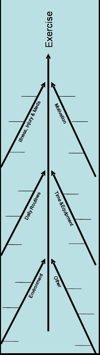
Figure 1:  A Sample Daily Page for Exercise

The back-page includes a Fishbone Diagram to assist the client in thinking through various causes of their behavior.  On the right of the page, clients can list the key causes they want to monitor for the next 2 weeks.  The creation of Fishbone Diagram and listing of causes to track is done prior to start of the diary entries.  This section of the back-page can be seen when looking at the daily page.  Figure 2 shows a sample back page organized for listing causes of exercise:

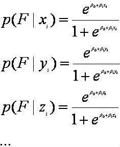
The client uses the diary for 2-3 weeks to monitor the occurrences of causes listed in the back page.  Once the diary is complete, they mail it to their clinician who analyzes the data and returns it to the client.  Repeated cycles of data collection and analysis allows the client and the clinician to understand what leads to success.  This diary is in use in a current research project of Moore and Alemi.

Definition of Terms Used in Analysis of Diary Data

Before we can show how the diary data should be analyzed, we need to define various terms and our abbreviations.  Assume that a client has collected daily information about presence of various causes X_i,Y_i,Z_i,... where X, Y and Z show the cause and "i" indicates the day.  The function X_i is 1 if the cause has occurred on day "i," and 0 otherwise.  Furthermore, suppose that we have also collected data on whether the client has failed or succeeded.  Let the function F_i be one if the client has failed on day "i," or 0 otherwise. 

The probability of failure given each cause is shown as p(F|X), p(F|Y), p(F|Z) and so on.  In this notation the vertical bar is read as "given" and the term "X" means a situation where the cause X is present and no other cause is present (X=1, Y=0, Z=0, ...).  We have for ease of presentation have deleted the explicit indication that all other causes should be absent.  p(F|X) is not the same as p(F|X, Y=?, Z=?, ...).  The former indicates the probability of failure from cause X given that we know nothing about occurrence of other causes.  The later shows the probability of failure given that cause X has occurred and no other cause has occurred.  The difference is that we know other causes have not occurred.  When people talk of the impact of cause, they are thinking of p(F|X), even though there maybe many causes that they are not aware of.  Part of the problem of analyzing diary data is to separate the impact of cause X from all other causes.  Statisticians typically refer to this as the main effect of the cause. 

We show the combined impact of X and Y and no other cause on the failure rate as p(F|X and Y).  When the number of causes examined is large, there are many potential interactions among them.   For example, if 3 causes (X, Y, and Z) are being tracked in the diary, the following interactions are possible:

p(F|X and Y)
p(F|X and Z)
p(F|Y and Z)

p(F|X, Y, and Z)

Examination of interactions between causes is important because of a special type of causes that we call constraints.  When a cause eliminates the impact of another cause, we refer to it as a constraint.  The constraint by itself has no impact on failure.  For constraint Y this is shown as:

p(F|Y) ≈ 0

In this equation "≈ 0" should be read as "is negligible or near zero."  Constraints interact with causes in reducing the probability of failure.  If X is a cause and C is a constraint, we show this as

p(F|X)>0

p(F|X and C) ≈ 0

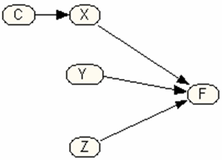
These two statements say that the impact of cause X on failure rates is reduced to a negligible amount because of the presence of constraint C.  A key task for analysis of diary data is to estimate the interactions among constraints and causes. 

Figure 3 visually shows the main effects for the three causes X, Y and Z and one Constraint C.  This Figure is a causal model.  It shows a network linking causes to failures.  A causal model should not contain a loop. i.e. it should not be possible to start from a node and follow the directions in the network and return to the same node.  The network of relationships depicted in Figure 1 does not include a loop.  It show how various causes and constraints affect the failure rate.  Each cause by itself is shown as a node.  The arcs between any two nodes show presence of an association.  In this Figure, no relationship is assumed between causes X, Y and Z.  The arrows show the direction of causality.  The effect of X is shown as an arrow from the node X to node F, the node marking failure.  The constraint C is assumed to affect the impact of cause X.  In the graph this is show as a directed link between constraint C and cause X.  The numerical relationship between C and X (not shown in the graph) is specified so that presence of C eliminates consideration of X as a cause of failure.

Figure 3:  A Causal Diagram Showing Causes X, Y and Z and Constraint C

Analysis of Diary Data

The analysis of diary data starts with making a few assumptions to simplify the task.  First, we list the causes and link them to the node marking failures.  Sometimes, at start of data collection, clients list causes that are so rare they never occur during the 2-weeks diary keeping.  These causes are not included in the analysis.  Other times, two causes always co-occur with each other in every data entry.  These two causes cannot be distinguished through data analysis and before proceeding a new cause that reflects the combination of the two is defined and used in the analysis.

When several causes are listed in a model, it is generally assumed that various combination of these causes must be estimated to verify the impact on failure rate.  Though this is not shown visually in the causal model, we assume that the impact of combination of causes is estimated by the sum of the impact of its components and therefore we are only estimating the main effects.  For example, for three causes X, Y and Z, we assume that:

p(F|X and Y) = p(F|X) + p(F|Y)
p(F|X and Z) = p(F|X) + p(F|Z)
p(F|Y and Z ) = p(F|X) + p(F|Y)
p(F|X, Y, and Z) = p(F|X) + p(F|Y) + p(F|Z)

Second, we list the constraints and draw an arrow from the constraints to the affected causes.  Note that in the diary depicted in Figure 2, we asked the client to identify the constraints prior to data collection.  Thus the clients insights can be used to list the constraints that should exist in the causal model. In Figure 3 we have listed one constraint: C.  It affects cause X. 

Third, each node is written as a function of its immediate preceding nodes.  For the Figure 3, this suggests two functions one for p(F|X, Y, and Z) and another for p(X|C).  For more complicated models, there would be additional separate functions. 

The law of Total probability states that the effect of several mutually exclusive causes is the weighted sum of the impact of each cause:

p(F|X, Y, Z, ...) = ∑_{I=X, Y, Z, ...}p(F|I) p(I)
Where p(I)=1 if cause I is present and otherwise 0

This is read as "probability of failure is a weighted linear sum of failure from various causes."  For example, the effect of the three causes on failure rates in Figure 3 is given by:

p(F|X, Y, and Z) = p(F|X) p(X) + p(F|Y) p(Y) +p(F|Z) p(Z)

The probability of cause X as a function of constraint C is expressed as:

p(X)= C X
X=1 if cause X is present and 0 otherwise,
C=1 if constraint C is present and 0 otherwise

Note that this function is 0 when both constraint C and the cause C are present.  The probability of failure as a function of both causes and constraints is obtained by substituting terms into one equation.  For Figure 3 this is calculated as:

p(F|X, Y, Z, and C) = p(F|X) CX + p(F|Y) p(Y) +p(F|Z) p(Z)

Fourth, the various probabilities are estimated so that the fit between the data and causal model is maximized.  A simple method to do so and which utilizes widely available statistical packages is to use logistic regression to fit the data to the causal model.  First, whenever a constraint is present the indicator variable for the affected cause is corrected and set to 0.  In logistic regression, the log of the odds of failure is regressed on the remaining variables X_i,Y_i, Z_i, and so on.

Log [p_i /(1-p_i )] = β₀x_i,+β₁y_i,+β₂z_i + ...+ ε_i

In this regression equation, p_i  shows the probability of failure in case "i."  If there are n weeks of data entry, then i=1, 2, 3,..., 2n.  The terms x_i, y_i, z_i ... are the i^th corrected diary entry for causes X, Y, Z and so on.  These variables are known and read directly from diary entries.  When the cause is present the variable is set to 1, when it is absent it is set to 0.  It is corrected in the sense that if in a particular day both the cause and the constraint are present, the indicator is changed from 1 to 0.  The coefficients β₀, β₁, β₂, ... are unknown parameters and estimated from the data.  The term ε_i is a residual random variable which cannot be observed.  It is assumed to have a mean of zero and a stable variance over time.  If most of data are explained by ε_i, or if the distribution of this variable is not random with mean of 0, then causes and constraints other than those listed in the diary are affecting failure rates.  Using the coefficients estimated in logistic regression, the various conditional probabilities of failure, the main effect of the cause on failure, can be calculated as:

Often the causes co-occur.  This is a by product of the fact that if the client finds a pattern of circumstances that works for the client, they are likely to repeat it.  This leads to situations where the various causes co-occur and therefore assessment of their contributions to failure rate will be affected by the nature of co-occurrences.  In causal modeling this leads to situations where there are also links among the causes as one cause can be used to predict the co-occurrence of another.  As a consequence of co-occurrences of causes, the order of entry of causes in the logistic regression affects the estimated variables.  Variables that are entered into the model first explain some of the variance in the failure rates and all other variables entered subsequently can at best explain only portion of the variance not yet explained.  Since, most causal inferences are exchangeable, in the sense that the order of occurrence of the cause has no effect in the net effect of the causes on failure rate, then logistic regression can be used to obtain two estimates for the main effects.  First, the variable is put into the equation first and a maximum estimate is obtained.  Then the variable is put into the logistic regression last and a minimum estimate is obtained.  The range of the maximum to minimum estimates is then presented to the client. 

Example

Suppose we have collected the diary data in Table 1.  This client had hypothesized three activities may further help keeping a morning exercise routine.  First was if the client would commute to work by bike and therefore exercise on route.  The second was if the client would take morning showers in the gym, thereby increasing the frequency of visits to the gym.  The last was to sleep early.  The diary also includes rainy days, which are expected to reduce the possibility of biking to work. 

The causes in the example in Table 1 can be mapped to the causal map in Figure 3.  Assume that constraint C is rainy day, cause X is plan to commute to work, cause Y is plan to take showers at GYM and cause Z is sleep early.  Note that rainy day is assumed to affect exercise by biking to work.  The corrected data is shown in Table 2. 

Using the corrected client's data in Table 2, we ran two logistic regressions for each cause.  The first had the cause as the first variable in the model and the second had it as the last variable in the model.  This produced maximum and minimum estimates fo the conditional probabilities (see Table 3).

	Maximum Logistic Regression		Minimum Logistic Regression		Probability of Failure Given the Cause
Cause	Constant	Coefficient	Constant	Coefficient	Minimum	Maximum
Plan to commute with bike
Plan to shower at GYM
Sleep early
Table 3:  Minimum & Maximum Estimates of a Cause Leading to Exercise Failure

Communicating to the Client

Typically analysis of diary data is done by an external group and communicated back to the client.  Most clients do not need to know how the estimates of impact of various causes were arrived.  The report to the client needs to focus on findings and not methods.  The report will provide the following information:

1. Advantages of keeping a diary over intuitive judgments
2. Description of causes analyzed. 
3. Limitations of the analysis
   • Not all causes of failure are known or were monitored
   • The impact of a cause on failure rate may change over time, making analysis of current data irrelevant to future patterns
4. List of causes found to affect failure rates in order of impact
5. Variation explained by all causes examined
6. Next steps

Before meeting with the client or sharing the data with the client it is important to ask the client to check the data by presenting to the client frequency of the causes and patterns of association between the cause and cause.   Frequency of occurrence of various causes are presented as a bar graph.  The association between the cause and failure rate is presented as visual table, where cell values are replaced by a variable circle marking co-occurrence among the failure rate and the cause. 

The data are presented in person to the client, allowing open question and answer periods. The presentation session is schedule ahead of time and well in advance.  A paper report is provided prior to the meeting.  The client is asked to anticipate rank order of causes in predicting failure rate prior to receiving the report.   No personal information appears on the written report in order to make sure that client's identity is not inadvertently revealed. 

At the meeting the client is reminded of the confidentiality of the findings and that the results are for sole use of the client.  A brief introduction is made of the team doing the analysis and goals of the analysis.  Limitations of diary data are highlighted.  The client is told that the purpose of putting numbers on impact of causes is to help produce insights in the exercise process.  The focus should be on improvement and not measurement. The data are presented without any blame or exhortation for the client to be more committed.  The client is told the purpose is not to understand how the environment affects the client's motivation and not asking the client to do more or be more motivated.  Findings are presented sequentially and after each section there is a pause to allow clients to ask relevant questions.  During the presentation no attempt is made to defend the validity of the diary approach or methods of analysis -- if clients are interested in these issues the topics are discussed in separate session.  At end of presentation of the findings, client is asked to indicate how findings will be used.  Furthermore, the client is asked to generate another set of causes to monitor for the next period of diary keeping.  

After the meeting a  cumulative lessons learned from various periods of data collection is mailed to the client along with a revised diary to be used in subsequent periods. 

References

Ahn WK, Kalish CW, Medin DL, Gelman SA. The role of covariation versus mechanism information in causal attribution. Cognition. 1995 Mar;54(3):299-352.

Alemi F, Alemi R.  A Practical Limit to Trials Needed in One-Person Randomized Controlled Experiments.  Quality Management in Health Care 2007.

Billing E, Bar-On D, Rehnqvist N. Causal attribution by patients, their spouses and the physicians in relation to patient outcome after a first myocardial infarction: subjective and objective outcome. Cardiology. 1997 Jul-Aug;88(4):367-72.

Cherpitel CJ, Bond J, Ye Y, Borges G, Room R, Poznyak V, Hao W. Multi-level analysis of causal attribution of injury to alcohol and modifying effects: Data from two international emergency room projects. Drug Alcohol Depend. 2006 May 20;82(3):258-68. Epub 2005 Oct 27.

Green TD, Bailey RC, Zinser O, Williams DE. Causal attribution and affective response as mediated by task performance and self-acceptance. Psychol Rep. 1994 Dec;75(3 Pt 2):1555-62.

Jaffe SL. Treatment and relapse prevention for adolescent substance abuse. Pediatr Clin North Am. 2002 Apr;49(2):345-52.

Kadden RM. Is Marlatt's relapse taxonomy reliable or valid? Addiction. 1996 Dec;91 Suppl:S139-45.

Kinderman P, Kaney S, Morley S, Bentall RP. Paranoia and the defensive attributional style: deluded and depressed patients' attributions about their own attributions. Br J Med Psychol. 1992 Dec;65 ( Pt 4):371-83.

Ladd ER, Welsh MC, Vitulli WF, Labbe EE, Law JG. Narcissism and causal attribution. Psychol Rep. 1997 Feb;80(1):171-8.

Larimer ME, Palmer RS, Marlatt GA. Relapse prevention. An overview of Marlatt's cognitive-behavioral model. Alcohol Res Health. 1999;23(2):151-60.

McKay JR. Studies of factors in relapse to alcohol, drug and nicotine use: a critical review of methodologies and findings. J Stud Alcohol. 1999 Jul;60(4):566-76.

Olsson J, Terris D, Elg M, Lundberg J, Lindblad S. The one-person randomized controlled trial. Quality Management in Health Care. 2005 Oct-Dec;14(4):206-16.

Pe'er D. Bayesian network analysis of signaling networks: a primer. Sci STKE. 2005 Apr 26;2005(281):pl4

Presentations

The narrated lecture in this section can also be followed on YouTube.com in three parts:

Part one:  people have different reason for why they exercise

 

Part two:  sample data from a diary & problems in analysis of diary data

 

Part 3:  Analysis of diary data using artificial intelligence methods