HAP 525:
|
||||||||||||||||||||||||||||||||||
|
Events
|
Probability
density function
|
Cumulative
distribution function
|
|
0 medication
errors
|
0.90
|
0.90
|
|
1 medication
error
|
0.06
|
0.96
|
|
2 medication
errors
|
0.04
|
1
|
|
Otherwise
|
0
|
1
|
Table 1: Examples of Probability Density and Cumulative Distribution Functions
Probability density function can be used to calculate expected value for an uncertain event. The expected value is calculated by multiplying the probability of the event by its value and summing across all events.

Where p(x=i) is the probability of event i
For the data in Table 1, the number of medication errors are sorted and listed to the left. The first column shows the probability density function. At each value, it provides the probability of the event listed. For example, 90% of patients have no medication errors, 6% of patients have 1 medication error and 4% have 2 medication errors. To calculate the expected value, first we multiply the value of each event by its probability. In the first row of Table 2, 0 medication errors is multiplied by 90% chance to obtain 0. In the second row, 6% is multiplied by 1 to obtain 0.06 and 4% is multiplied by 2 to obtain 0.08. The expected medication error is the sum of the products of the event value and its probability. In this example it is 0.12..
|
Events
|
Probability
density function
|
Value times
probability
|
|
0 medication
errors
|
0.90
|
0
|
|
1 medication
error
|
0.06
|
0.06
|
|
2 medication
errors
|
0.04
|
0.08
|
|
Otherwise
|
0
|
0
|
|
Total
|
0.12
|
Table 2: Calculation of Expected Medication Errors
Knowing the probability density function is a very important step in deciding what to expect. Naturally, a great deal of thought has gone into recognizing different probability distributions. The most common density probability functions for discrete variables are Bernoulli, Binomial, Geometric, and Poisson functions. We will describe each of these functions and explain the relationships among them. These functions are useful in describing a large number of events, for example the probability of wrong side surgery, the time to next gun shot in a hospital, the probability of medication errors over a large number of visits, the arrival rate of security incidences and so on. If our focus remains on events that either happen or do not occur, then these four distributions are sufficient to describe many aspects of these events.
Bernoulli density function is the foundation often used to construct more complex distribution functions. It assumes that two outcomes are possible. Either the event occurs or it does not. In other words the events of interest are mutually exclusive. It also assumes that the possible outcomes are exhaustive, meaning at least one of the outcomes must occur. In a Bernoulli density function, the event occurs with a constant probability of p. The complement event occurs at probability of one minus p.
f(Event occurs) = p
f(Event does not occur) = 1-p
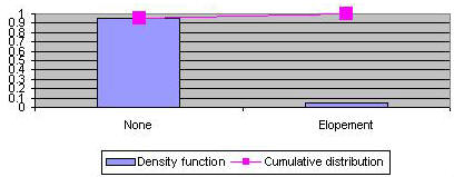
Typically, it is assumed that the probability is calculated for a specific number of trials or a specific period of time. For example, Figure 1 shows the density and cumulative distribution function for a facility where patients have a 5% chance of elopement per day.

Figure 2: Example of a Bernoulli Density and Cumulative Distribution Function
Lets now think through a situation where a Bernoulli event is repeatedly tried. Lets assume that in these trials the probability of occurrence of the event is not affected by its past occurrence, in other words that each trial is independent of all others. When we are dealing with independent repeated trials of Bernoulli events, a number of common density functions may describe various events. For example, the time to the first occurrence of the event has a Geometric distribution. To help you think through why that is the case, lets start with looking at an example of repeated independent trials.
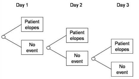
In this situation we have 3 repeated trials for tracking patients elopement over time (see Figure 3). We are assuming that the probability of elopement does not change if one patient has eloped in the prior days. In day 1, the patient may elope or not. In day two, the same event may repeat. The process continues until day three. As you can see the patient may elope in different days and on each day this probability of elopement on that day is constant and equal to values on prior days. Independence cannot be assumed for all repeated trials. For example, probability of contagious infection changes if there was an infection in the prior day. Therefore, independent trials cannot be assumed in this situation. But in many situations it can and when we can there is a lot we can tell about the probability function under this assumption.

Figure 3: Repeated Trials
If a Bernoulli event is repeated until the event occurs, then the number of trials to the occurrence of the event has a Geometric distribution. The Geometric density function is given by multiplying probability of 1 occurrence of the event by probability of k-1 non-occurrence that should precede it.
f(k) = (1-p)k-1p
An interesting property of Geometric probability density function is that the expected number of trials prior to occurrence of the event is given by dividing 1 by the probability of the occurrence of the event in every trial:
Expected number of prior trials = 1/p
As we will see later, this fact is used to estimate probability of rare events that might occur only once in a decade. If an event has occurred once in the last decade, then the daily probability of the event is 3 in 10000, a very small probability indeed.
In repeated independent trials of Bernoulli event, the Binomial density function gives the probability of having k occurrences of the event in n trials. Take the repeated trials in Figure 3, there are several ways for having 2 patients elope in 3 days: patients elope in days 1 and 2 but not 3, patients elope in days 1 and 3 and not 2, or patients elope in days 2 and 3 and not 1. In all three instances, the probability is p2 (1-p) but the days in which the patients elope are different. To properly account for number of possible ways of arranging k items in n possible slots, we need to use a combinatorial. This is why the binomial density function looks like the following:
![]()
In this formula, n! is referred to as n factorial. A factorial of a number is equal to product of all numbers less than it, i.e. it is equal to 1*2,*3, ...., *(number-1)*number. The proportion n! / [k! (n-k)!] counts the number of different ways k occurrence of an event might be arranged in n trials. The term pk measures the probability of k occurrences of the event and the term (1-p)n-k measures the probability of n-k non-occurrence of the event.
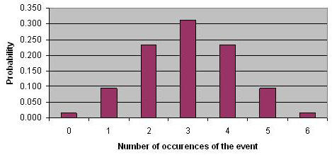
Figure 4 provides an example density function for Binomial distribution based on repeated independent Bernoulli trials with probability of 1/2. In this Figure, you see a Binomial distribution with 6 trials. There are seven possibilities. Either the event never occurs or it occurs once, twice, three, four, five, or six times. The probability density function shows the likely occurrences. The most likely situation is for the event to occur three times in 6 days. This is also the expected value and can be obtained by multiplying the number of trials by the probability of occurrence of the Bernoulli event. Note that the distribution is symmetric, though as we will see shortly when p value is less than 0.5 then the distribution gets skewed to the left.

Figure 4: Binomial Distribution for Repeated Independent Bernoulli Functions with p=1/2
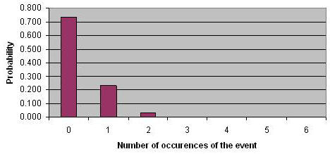
Lets now go back to the patient elopement example, where the daily probability of elopement was 5%. Over a 6 day period, we are most likely to see no patients elope (see Figure 5). There is a 23% chance of seeing one elopement and there is a 3% chance of seeing two elopements. Note how the distribution is skewed to the left. This is always the case when p is less than 50%. The more it is smaller than 50% the more it would be skewed to the left.

Figure 5: Binomial Distribution for Repeated Independent Bernoulli Trials
with p=0.05
In a Binomial distribution, the expected value is calculated from the following formula:
E(occurrence of the event) = np
Where n is the number of trials and
p is the probability of occurrence of the event in one trial
Now we can answer questions such as how many patients might have an adverse effect in a defined period of time. For example, if the daily probability of elopement is 0.05, the expected number of elopement over a year is 0.05*365 = 18.25 persons.
As the number of trials increases and the probability of occurrence drops, Poisson distribution approximates Binomial distribution. In risk analysis, this occurs often. Typically we are looking at a large number of visits or days and the sentinel event has a very low probability of occurrence. In these circumstances, the number of occurrence of the event can be estimated by Poisson density function:

In this formula, Lambda is the expected number of trials and is equal to n times p, where n is the number of trials and p is the probability of the occurrence of the event in one trial. Furthermore, k is the number of occurrences of the sentinel event and e is 2.71828, the base of natural logarithms. Poisson distribution can be used to estimate number of sentinel events over a large period of time.
To assist you in reviewing the material in this lecture, please see the following resources:
Listen to narrated lecture on calculating hazard functions. See the slides for the lecture
Listen to part one of the lecture on
probability distributions:
Narrated lectures require use of Flash.