 |
 |
Evaluating Programs: Measuring Impact of Programs on Patients' Satisfaction and Health Status |
|||||||||||||||||||||||||||||||||||||||||||||||||||||||||||||||||||||||||||||||||||||||||||||||||||||||||
IntroductionThis section introduces you to program evaluation. In particular, we show you how to set up a data collection procedure that will allow you to examine the impact of changes in practice patterns on patient outcomes. The ideal approach is to organize a random experimental design, where in patients are randomly assigned to control and experimental groups. This is difficult to accomplish. An alternative approach is to use principles of quasi-experimental design and statistical process control tools to examine programs. While this approach is less accurate than random experimental design, it is easier to implement and provides a reasonable protection against bias. This approach is the focus of this section. . In evaluating outcomes, you have to decide what outcomes you want to measure. There are many possibilities including specific morbidity and mortality. Since most small scale program evaluations can not detect statistical differences in mortality, alternative measures are needed. One alternative is to measure patients' satisfaction with the care. While patient satisfaction does not adequately measure the clinician's knowledge and effectiveness, it does provide a reasonable measure the care with which it was delivered. From a business point of view, satisfied customers are more likely to return for additional services. This section discusses how to measure patient satisfaction. Another way to measure outcomes is to ask the patients to report their health status. This section introduces you to how to measure self reported health status. There are many ways to measure health status. One increasingly popular approach is to ask patients about their health. A good example of a questionnaire that does so is the SF-36 questionnaire. This is a 36 item questionnaire that has proven to be reliable in numerous studies. This session focuses on the SF-36 questionnaire. This section ends with a detailed discussion of the pitfalls of evaluating outcomes. In small studies, there is always a danger of attributing patient outcomes to changes in our care when in fact such outcomes may be due to some external co-occurring change. Many clinicians make a change and see the associated improvement patient outcomes and claim that their change has led to improvement. Interpreting a causal relationship between change and patient outcomes based on the association between these two is akin to reporting that firemen cause fire because they are often present when houses burn. We discuss in some detail how evaluating patient outcomes could lead to erroneous conclusions and what we need to do to protect against these biases. Objectives
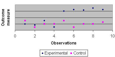
Evaluating Changing ProgramsThere are a number of different methods for program evaluation.[1] The ideal method of program evaluation is to randomly assign patients to control and experimental groups and evaluate, change the care of the experimental group and examine if there is a difference in patient outcomes in the two groups. This ideal is seldom achieved. There are several difficulties. First, it is difficult and at times unethical to randomly assign patients to providers, as patients would like to make their own choices. Second, and perhaps more important, providers like to tinker with their care and improve it continuously. The ideal program evaluation requires that during the course of the evaluation we keep the care constant. Since program evaluation takes months to complete, this requirement is onerous and makes ideal program evaluation difficult. Many evaluations go unused both by those evaluated and by those for whom the evaluation was completed.[2],[3] The longer the evaluation, the more artificial the restrictions in the evaluation (e.g. holding programs constant or randomly assigning clients to providers), the less likely that providers will feel that it reflects their care. In these circumstances, providers may ignore evaluation results -- even though they have been painstakingly put together to protect against external biases. We recommend the use of continuous quality improvement in conducting program evaluation, a process we call Continuous Improvement Evaluation.[4] While it does not provide the protections available in the ideal evaluation design, it provides timely and relevant data to providers of care. It does not require programs to stop from innovating and changing. Evaluation results are available in an on-going basis. The evaluation itself changes little in care operation and thus it is more compatible with on-going activities. Data are collected from both a control group as well as the program patients (experimental group). Data are collected over time before the start, during and after the end of the program. In the figure 2, we show data collected over 10 time periods. In addition, data should be calculated from medical records concerning severity of illness. The impact of the program on patient outcomes can be assessed by comparing observed patient outcomes to expected outcomes (typically established from the patients' severity of illness or from the patients patterns prior to recent program changes).
Figure 1: Data Collected from Two Groups Over Time Patients can be recruited into the programs by writing to individuals before they come for care, while seeking care or after care. In all instances, a consent is needed for further contact to explain the evaluation effort. Evaluation MeasuresThe first step is to clarify the program objectives and identify key measures for each objective. The process measure will gauge program effort and outcome measures will identify the impact of the program. Program evaluation could have different focus {See Table 1}. It can examine the approval of the program and enrollment of the patients. It can contrast what was done to what should have been done. It can examine the market share and demand for a program. We prefer to focus on patient outcomes and by these we mean mortality, morbidity, satisfaction with care, and patient self report of their own health status.
Table 1: Possible Measures of Program Outcomes Patient SatisfactionReaders may prefer to focus on clinical outcomes as opposed to patient satisfaction. The measures of patient satisfaction is often reasonable because (1) It give customers a voice - which is often effective strategy in changing provider patterns, (2) It evaluate care from the customer’s own values, (3) It measure facet of care not easily examined, including compassionate bedside skills, efficient attendance to needs, participation in decision-making, adequate communication and information to patients. Patient satisfaction is also of concern from a business perspective. It shows how likely is the patient to choose the same health care organization in the future and recommend it to his or her friends. As such, it is an early marker for changes in market share. Compared to clinical outcomes, patient satisfaction measures have following advantages:
Pascoe envisages patient satisfaction as healthcare recipients‘ reactions to their care. A reaction that is composed of both a cognitive evaluation and an emotional response. In this context, there are no right or wrong, all reactions are valid. Patients can legitimately be dissatisfied with care that everyone may consider great. To understand the meaning of patient satisfaction, we need to examine how individuals arrive at their judgments. Each patient begins with a comparison standard against which care is judged. Standard can be an ideal care, a minimal expectation, an average of past experiences, or a sense of what one deserves. The patient can assimilate discrepancies between this expected and actual care. What is not assimilated affects patient ratings of satisfaction. Thus patient satisfaction can be affected not only by the care but also by provider communications regarding what should be expected and by patients' attribution of who or what influenced the care. There are many examples of patient satisfaction instruments. One such index is the Patient Satisfaction Questionnaire (PSQ). Another is the Patient Judgments of Hospital Quality Questionnaire (PJHQ). The Medline database includes numerous other examples including instruments that are specific for different clinical areas. The PSQ instrument assess patient satisfaction on the following dimensions:
The Patient Judgment of Hospital Quality is based on the following dimensions:
You do not need to rely on existing instruments, you can create your own. We recommend that you rely on established instruments whose reliability and validity is known and for which benchmarks are available. In contrast if you do your own, you can include questions that may speak more directly to issues raised at your organization. To construct your own instrument follow these steps:
There are a number of problems with using satisfaction as patient outcomes:
One way to measure patient satisfaction is to measure time-to-dissatisfied customer. In the "time-to-dissatisfied customer" approach, sampled patients are asked one question at start which assesses the overall satisfaction with care. Patients with extreme responses are asked to complete a longer survey which is designed to understand reasons for dissatisfaction or high satisfaction. The typical first stage question appears like the following:
Figure 2: Sample First Stage Survey for Time-to-Dissatisfied Customer The second sample is asked from patients in the two extremes (delighted or not meeting minimum expectations). From these patients the survey asked for reasons for their reaction. At this point, an existing survey instrument can be used or an alternative instrument such as the following questions can be asked:
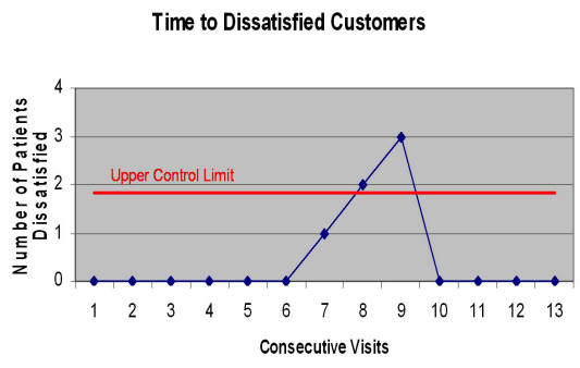
Both time-to-dissatisfied customer and average satisfaction of customers produce data that can be used to monitor process improvement. The responses from the first stage surveys of time-to-dissatisfied customer can be used to measure time to a visit with a dissatisfied customer. Time-between charts can be used to analyze the time-to-dissatisfied customer (see a sample output in Figure 4):
Figure 4: An example of how time-to-dissatisfied customer can be analyzed This graph shows the data for the last 13 visits. It shows that a statistically significant change occurred in visits 7, 8 and 9, where 3 consecutive patients were dissatisfied. Clearly, using the new control chart techniques, such as time between charts, it is possible to monitor changes in a work process. As mentioned earlier there are two advantages:
Measuring Health StatusPatients' health status is usually measured through clients' self report. Clients' are asked to report their ability to function and carry through with specific objective activities, such as climbing steps. There are not asked to describe their preferences for different life styles, which could be idiosyncratic. One advantage of the use of health status measures is that it is available on all diseases across all institutions, and therefore can be used to profile and compare providers care within and outside an organization. A number of instruments have been proposed for measuring patients' health status. These instruments are available in Medline and enable the assessment of quality of care in specific diseases. Prominent among these surveys are the SF-36 survey. Read more about SF-36 survey instrument (Requires Adobe file reader). The SF-36 is based on both physical and mental health. The physical health has four sub-components. These are (1) physical functioning, (2) Role limitation due to physical health problems. (3) Bodily pain and (4) General health. The mental health component also has four components. These are (1) Vitality (i.e., energy, fatigue), (2) Social functioning, (3) Role limitations due to emotional problems and (4) Mental health More than 4000 studies have used the SF-36. It is translated to more than 14 languages. Many of these studies show the validity of the instrument in differentiating among sick and well patients. With few exceptions, overall reliability of SF-36 exceeds 70%; a relatively high reliability that shows the instrument can be used for comparing groups of patients. The reliability of the eight scales in SF-36 is shown in Table 3:
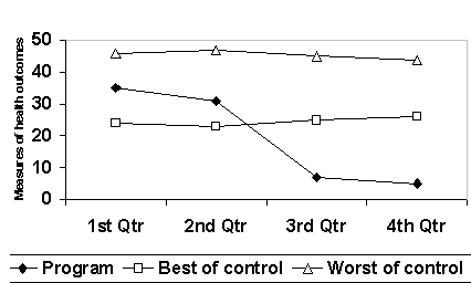
Methods of AnalysisWe can use statistical process control to trace the performance of the program over time. Thus, we will be able to answer whether changes in the program have led to statistically significant improvements over time. By studying the performance of the program over time, we are able to conduct a series of small-scale improvement studies as programs evolve. The most common design proposed by intervention programs is to collect data pre and post intervention. For a constantly changing intervention, more frequent observations are necessary to detect changes in the nature of the intervention that might have occurred between the pre and post-test data points. More frequent observation may at first seem onerous for the intervention staff; but it is not. For all practical purposes, we are collecting data over time from our patients. Even when some claim that they are collecting data before and after intervention, variations in client follow-up rates and staff scheduling limitations force collection of data over different time periods. In a four month follow-up study, for example, some patients may get their exit interview in 3 months while other patients may get the same interview in 5 months. Difficulty in recruiting clients at same time period leads to recruitment schemes that are over time. Some clients may receive the early intervention and other clients may receive a more mature intervention six months later. Collecting data over time is something that intervention programs are already doing. What we are proposing is to explicitly recognize what is already implicitly part of many evaluation studies. Cook and Campbell recommend use of interrupted time series over pre and post test studies as the strongest method of conducting quasi-experimental designs for evaluation studies.[9] To control for potential interaction of extraneous events and intervention effect, they encourage use of a time series from comparison sites. In a similar fashion, we propose to use statistical process control tools, in which the outcomes of one locality are traced over time and compared to outcomes of a mix of other sites. This design provides strong protection against threats to validity, similar to the interrupted time series design recommended by Cook and Campbell. In conducting the analysis, first expected process limits are calculated. These limits are based on data patterns in either the control group or patterns of severity of illness of patients in the experimental group. Then the rates observed in the experimental group are compared to the expected limits. If observed rates fall within the expected upper and lower limits (the so called best and worst of the control group), then the program outcomes have not changed. If they fall outside the limits, then the program has made a statistically significant change compared to the control group. Figure 5, for example, shows how data collected over time from control and experimental groups can be displayed to highlight changes due to program improvements.
Figure 5: An example of Use of statistical process control tools for program evaluation In the figure above, the X-axis shows time. The Y-axis shows a measure of impact, for example percent patients immunized or percent patients satisfied. The line titled 'best of control group" is the Upper Control Limit for similar cases in control sites. This is a line that is three standard deviations away from the average of similar cases in the control group. The line titled "worst of control group" shows the Lower Control Limit for similar cases among control sites. When program data are within upper and lower control limits (best and worst line), then the program is performing statistically like the control group. When program data are below the lower control limit, then it is outperforming similar cases in control sites. In this example, in the first two quarters the program's data are within limits but in the last two quarters the program is outperforming similar cases in the control sites. Statistical process control charts allow both comparison of the program to comparison sites as well as to itself over time. In this sense, it provides a robust study design. In order to make sure that each program is compared to similar sites, each control site is weighted according to its similarity to target program site. This method of analysis uses the concept of risk-adjusted statistical process control used previously in monitoring falls in nursing homes,[10] diabetes patients in control, [11] and hospitals rate of mortality from myocardial infarctions.[12] The formulas for calculating upper and lower control limit from the data of patients in the control group is given as follows:
In the above formula, O marks the average expected outcome. S designates the standard deviation. The number of cases in the control group is m. For each case j in the control group, we calculate a weight W that measures the similarity of the case to the average case in the experimental group. In addition, for each case j in the control group we measure the outcome O. A key element of the methodology is how we weight similar cases. Psychologists have conducted numerous experiments showing that similarity of two individuals will depend on features they share and features unique to each case.[13]-[17] Features in a case can be demographics (e.g. gender, age, ethnicity), specialization, employment status, board certification, prior training in bioterrorism or other characteristics. Tversky (1977) summarized the research on similarity and provided a mathematical model for judgments of similarity.[18] We use the formula suggested by him and supported by research conducted by psychologists (see footnote for detailed procedures[19]). Potential Limitations[20]The following discusses a variety of threats to validity of Continuous Improvement Evaluation. In each case, we begin with the statement of the potential threat and follow by how the proposed approach addresses the threat. Potential threat of poorly defined populations.
Typically a well-defined study population is required to control for extraneous
influences and to create a homogeneous sample in which to perform the
evaluation. For example, patients may have significant differences in age,
preparedness, organizational experience and other characteristics. In addition,
providers work for organizations that may have significant differences in
budget, external threats, culture and other characteristics. It is not
reasonable to compare patients and organization with such differences to each
other. To do so would be akin to comparing apples to oranges. Potential threat of treatment contamination.
Typically one expects that well-defined interventions be used to address
construct validity and to protect against diffusion, contamination and imitation
of treatments by the comparison groups. This ensures that any "significant"
difference can indeed be ascribed to a specific intervention. For example it is
possible that early success of one organization may be copied by other
organization and therefore the diffusion of the innovation makes it difficult to
detect its impact. For another example, it is possible that cycles of
improvement will lead to changes in the program making it difficult what is
being evaluated. Potential threat of poorly defined control group.
Typically control groups are used to ensure that effects are not artificial,
and to distinguish true effects from temporal trends. Foremost among these are
maturation effects and regression to the mean. The threat is that the
change may occur anyway with or without the experimental intervention. .
In most quasi-experimental designs, an experimental group is compared to a control group, which receives usual care. Usual care is a euphemism as over time programs improve. There is no stable usual care. In the real world, every provider and every program is always changing. While these changes may introduce biases, study design allows for us to detect these potential problems in the data and correctly interpret the findings. Potential threat of baseline differences. Clients differ in their baseline values. Some
are at high risk and others are at low risk for incidence of adverse outcomes.
Interventions maybe effective at improving outcomes among high-risk patients but
still have lower outcomes than low risk patients do. In essence, the
argument is that where you end up, in
part depends where you started. To ignore these differences would brand
effective programs as useless. Potential threat of not having a replication. In
the Western scientific method, there is an absolute requirement for replication
of scientific findings. Even in the hard physical sciences, a scientific
"result" like cold fusion must be replicated in both the same or an independent
experiment. This becomes even more important in behavioral and social science
settings. Here, there is considerable variation among study subjects. Without
replication, it is impossible to refute the claim that any "result" was simply
due to chance variation among study subjects. In the proposed methodology, no
systematic replication seems to have been built into the design of the
experiment. The interventions are constantly changing through the CQI
paradigm. It is hard to see how one can refute the claim that any "result" was
simply due to chance variation, i.e., a "fluke." Consider for example the trivial example when the name of a program changes. Has the intervention changed? Perhaps not. No significant change has occurred until the outcomes of the intervention change. In the absence of such changes the intervention is a replication of last time period. Statistical process control examines outcomes over time to infer whether any time period is different from comparison sites or from previous time periods for the same site. Thus, it addressed whether the improvement is a "fluke" or real. When the improvement is real, then our hypothesis that the interventions have not really changed (i.e. they are replication of previous time periods) is rejected. What Do You Know?Advanced learners like you, often need different ways of understanding a topic. Reading is just one way of understanding. Another way is through writing. When you write you not only recall what you have written but also may need to make inferences about what you have read. The enclosed assessment is designed to get you to think more about the concepts taught in this session. PresentationsSelect one of the following presentations:
Narrated slides require use of Flash. References & MoreTesta, Marcia A. MPH, PhD; Simonson, Donald C. MD Current Concepts: Assessment of Quality-of-Life Outcomes. New England Journal of Medicine. 334(13):835-840, March 28, 1996. Accession Number: 00006024-199603280-00006 [1] Devine P., Christopherson E., Bishop S. (1996) Self-adjusting treatment evaluation model. Center for Substance Abuse Treatment Office of Scientific Analysis and Evaluation, Evaluation Branch, Washington DC. [2] Haines A., Jones R. (1994) Implementing findings of research British Medical Journal Jun 4; 308 (6942):1488-92. [3] Davis P., Howden-Chapman P. (1996) Translating research findings into health policy. Soc Sci Med; 43 (5): 865-72 [4] Alemi F, Haack M, Nemes S. Continuous Improvement Evaluation: A framework for multi-site evaluation studies Journal for Healthcare Quality, 2001, 23, 3, 26-33. [9] Cook T. D., Campbell D.T. (1979) Quasi experimentation: Design and analysis issues for field settings. Houghton Mifflin Company, Dallas. [10] Alemi F, Oliver D. Tutorial on risk adjusted p-charts. Quality Management in Health Care 2001, 9:4. [11] Alemi F, Sullivan T. Tutorial on Risk Adjusted X-Bar Charts: Applications to Measurement of Diabetes Control. Quality Management in Health Care 2001, 9:3. [12] Alemi F, Rom W, Eisenstein EL. Risk adjusted control charts. In Ozcan YA (editor) Applications of Operations Research to Health Care Annals of Operations Research, 67 (1996) 45 - 60. [13] Mobus C. (1979) The analysis of non-symmetric similarity judgments: Drift model, comparison hypothesis, Tversky's contrast model and his focus hypothesis. Archiv Fur Psychologie; 131 (2): 105-136. [14] Siegel P.S., McCord D. M., Crawford A. R. (1982) An experimental note on Tversky's features of similarity. Bulletin of Psychonomic Society; 19 (3): 141-142. [15] Schwarz G, Tversky A. (1980) On the reciprocity of proximity relations. Journal of Mathematical Psychology; 22 (3): 157-175. [16] Tversky A. (1977) Features of similarity. Psychological Review; 84 (4): 327-352. [17] Catrambone R., Beike D., Niedenthal P. (1996) Is the self-concept a habitual referent in judgments of similarity? Psychological Science; 7 (3): 158-163. [18] Tversky A. (1977) Features of similarity. Psychological Review; 84 (4): 327-352.
[19]
Calculation of weighted benchmarks: X = (∑i=1, …, N Oi )/ N At time "t", the similarity, Wij, between case "i" in the site and case "j" in the comparison group can be calculated by the formula: Wij = fi,j / [fi,j + a (fi, not j) + b (fnot i, j)] Where fij is the number of features shared between clinician "i" and "j"; fi, not j is the number of features of clinician "i" but not of clinician "j"; and fnot i, j is the number of features of clinician "j" but not of clinicians "i". The parameters a, and b are constants between zero and one and sum to one. In calculating upper and lower control limits, we weigh cases in the comparison groups based on their average similarity to clinician at the target program. Thus, Wj , the weight for case "j" in comparison group is calculated as: Wj = ∑j=1, …N Wij / N If at time period "t" there are "M" cases in the comparison site and if as before "Oj" shows the outcome for alumni "j"; then the weighted average of the outcomes at the comparison sites, O, is calculated as: O = (∑j=1, …, M Wj Oj)/ ∑j=1, …, M Wj The weighted standard deviation for the outcomes at the comparison site for time period "t" is calculated as: S = [∑j=1, …, M Wj (Oj - O)2/(-1+∑j=1, …, M Wj)]0.5 The upper control limit (UCL) at time "t", a point on the line marked the "Best of similar cases in comparison sites" in Figure 1, is calculated as: UCL = O + 3 S Similarly the lower control limit at time "t" is calculated as: LCL = O - 3 S [20] This discussion of threats follows the text of the article we published earlier on a similar topic. For more details see Alemi F, Haack MR, Nemes S. Continuous improvement evaluation: a framework for multisite evaluation studies. J Healthc Qual. 2001 May-Jun;23(3):26-33. [21] Read more on health status measurement. [22] See clearinghouse on measures of quality. [23] Read about health status of children. [24] Examine validity of SF-12. [25] Review of literature on satisfaction ratings More► |
|||||||||||||||||||||||||||||||||||||||||||||||||||||||||||||||||||||||||||||||||||||||||||||||||||||||||
|
This page is part of the course on Quality / Process Improvement. It was last revised on 01/15/2017 by Farrokh Alemi, Ph.D. |
|||||||||||||||||||||||||||||||||||||||||||||||||||||||||||||||||||||||||||||||||||||||||||||||||||||||||