 |
HAP 525:Risk Analysis in HealthcareWhat is Probability?
This is the first lecture on a series of lectures intended to prepare you to do probabilistic risk analysis. This lecture introduces the concepts of probability as a series of partitioning of the universe of possibilities. It also introduces you to axioms of probability and subjective methods of assessing probabilities from experts’ opinions. We quantify the probability of an event so that we can make tradeoffs among uncertain events, measure the combined impact of several uncertain event and communicate our uncertainty about future events to others. Probability quantifies how uncertain we are about a future events. A more formal definition of probability is to define it in terms of axioms from which the rest of the calculus of probability can be derived. If just four axioms are met then all of the calculus of probability are implied. These axioms are the following:
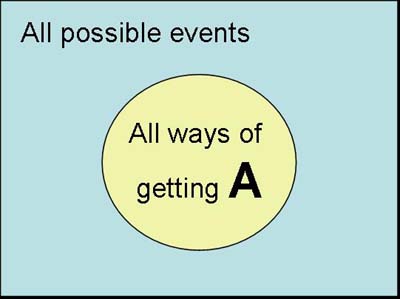
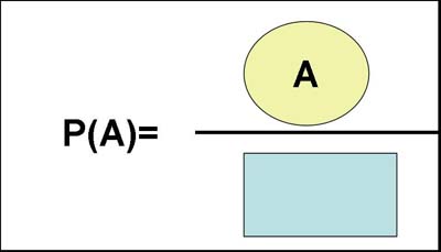
If numbers can be assigned to events such that they follow these four axioms, then the numbers are a probability function and follow the entire calculus of probability. The best way to think of probabilities is as the ratio of all ways in which an event may occur divided by all possible events. In short, probability is the prevalence of the event among the possible events. The probability of a small business failing is then the number of business failures divided by the number of small businesses. The probability of an iatrogenic infection in the last month in our hospital is the number of patients who last month had an iatrogenic infection in our hospital divided by the number of patients in our hospital during last month. When we are sure that an event will occur, we say that it has a probability of 1. When we are sure that an event will not occur, we assign it a probability of zero. When we are completely in dark, we give it a probability of 0.5, a fifty - fifty chance of occurrence. All other values between 0 and 1 measure how uncertain we are about the occurrence of the event. A Venn diagram shows the frequency of an event compared to the frequency of all possible events. The circle in Figure 1 shows the frequency of event A and the rectangle shows the frequency of all possible events. The blue portion of the rectangle shows the frequency of events that are not A occurring. Note how the sample space is the sum of the event and its complement. This is implied by the 1st and 3rd axioms. The first axiom requires the probability of the entire sample to be one. The third axiom requires that probability of the complement to be one minus probability of the event.
Figure 1: A Graphical Intuition for Definition of Probability So what is the probability of not A. Graphically, it is all the blue area with the hole in the middle divided by the square area. Logically it is the count of all events that are not A divided by all possible events. So what is the probability of no one having an iatrogenic infection in our hospital. It is the count of patients who do not have iatrogenic infection divided by total number of patients.
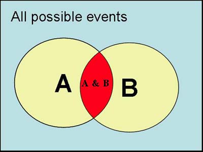
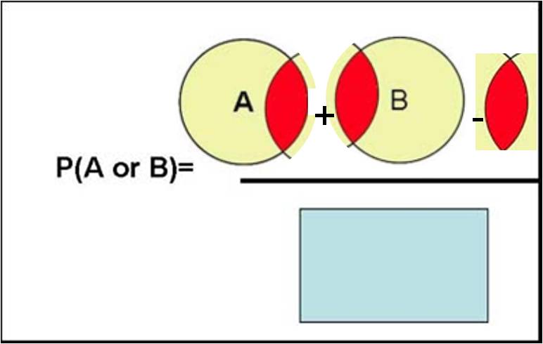
Top pf Figure 1 presents a Venn diagram. A Venn diagram shows the universe of possibilities, events and sometimes (though not usually) the elements. An element is the smallest unit of analysis. It is counted to construct events. For example, in analysis of medication errors visits may be considered an element. Events are a grouping of elements. For example, all visits in which a medication error has occurred may be considered the medication error event. A collection of all possible events is the universe of possibilities. The rules of probability allow us to calculate probability of combination of events using the above definition of probabilities. The probability of two events A and B occurring together, is calculated by first summing all the possible ways in which event A will occur plus all the ways in which event B will occur, minus all the possible ways in which both event A and B will occur (this term is subcontracted because it is double counted). This sum is divided by the all possible ways that any event will occur. This is represented in mathematical terms as: P(A or B) = P(A) + P(B) - P(A & B) Graphically, the concept can be shown as the yellow and red areas in Figure 2 divided by the blue area.
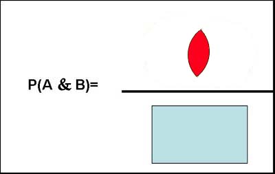
Figure 2: Graphical Representation of Probability of A or B Similarly, the probability of A and B occurring together, corresponds to the overlap between A and B and can be shown graphically as the red area divided by all possible events (the rectangular blue area) in Figure 3.
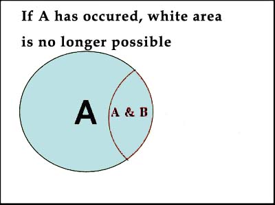
Figure 3: Graphical Representation of Probability A and B The definition of probability gives us a simple calculus for combining uncertainty of two events. We can now ask questions such as: "What is the probability that frail elderly (age>75) or infants will join our HMO?" According to our formulas this can be calculated as: P( Frail elderly or Infants join HMO) = Since the chance of being frail elderly and infant is zero (i.e. the two events are mutually exclusive), we can re-write the formula as: P( Frail elderly or Infants join HMO) = P( Frail elderly join HMO) + P( Infants join HMO) The definition of probability also helps us calculate the probability of an event conditioned on the occurrence of other events. In these circumstances, we know something has happened and we are asking for the calculation of the probability of another event. In mathematical terms we show this as P(A | B) and read it as probability of A given B. When an event occurs, it reduces the remaining list of possibilities; we no longer need to track the possibility that the event may not occur. We can use our definition of probabilities to calculate conditional probabilities by restricting the possibilities to only events that we know have occurred. Graphically, this is shown as in Figure 4.
Figure 4: Probability of B Given A is Calculated by Reducing Possibilities For example, we can now calculate the probability that a frail elderly joins the HMO and is hospitalized. Instead of looking at hospitalization rate among frail elderly, we need to restrict the possibilities to frail elderly who have join the HMO. Then the probability is calculated as the ratio of hospitalization among frail elderly in the HMO to number of frail elderly in the HMO. For another example, consider that an analysis has produced the following joint probabilities for the patient being in treatment or in probation:
Please note that table 1 provides joint and marginal probabilities by dividing the observed frequency of days by the total number of days examined. Marginal probabilities refer to the probability of one event. In Table 1 these are provided in row and column named "total." Joint probability refers to the probability of two events co-occurring at same time. In Table 1, these are provided in the cell values not labeled as "Total." For example, the joint probability of having both probation and treatment day is 0.51. This probability is calculated by dividing the number of days in which both probation and treatment occur by the total number of days examined. The total number of days is referred to as the universe of possible days. If the analyst wishes to calculate a conditional probability, the total universe of possible days must be reduced to days with the condition. Suppose the analyst wants to calculate the conditional probability of being in treatment given that the patient is already in probation. In this case, the universe is reduced to all days in which the patient was in probation. In this reduced universe, the total number days of treatment is the number of days of having both treatment and probation. Therefore, the conditional probability of treatment given probation is: p(Treatment day | Probation day) = Since Table 1 provides the joint and marginal probabilities, we can describe the above calculations in terms of joint and marginal probabilities by dividing the top and bottom of the above division by the total number of possible days: p(Treatment day | Probation day) = P(Both treatment and probation) / p(Probation) p(Treatment day | Probation day) = 0.51/0.56 = 0.93 The point of this example is that conditional probabilities can be calculated easily by reducing the universe examined to the condition. You can calculate conditional probabilities from marginal and joint probabilities if you keep in mind how the condition has reduced the universe of possibility. Conditional probabilities are a very useful concept. They allow us to think through an uncertain sequence of events. If each event can be conditioned on its predecessor, a chain of events can be examined. Then if one component of the chain changes, we can calculate the impact of the change through out the chain. In this sense, conditional probabilities show how a series of clues might forecast a future event. The point of this introduction has been that the calculus of probability is an easy way to track the overall uncertainty of several events. The calculus is appropriate if several simple assumptions are me. These include the following:
If a set of numbers assigned to uncertain events meet these three principles, then it is a probability function and the numbers must follows the algebra of probabilities. Odds & ProbabilitySome people prefer to describe their uncertainty about an event in terms of odds for the event occurring and not use the concept of probability. The two concepts are related. Odds are expressed as ratios while probabilities are expressed as decimals between 0 and 1. The odds for an event is related to its probability by the following formula:
For example, if the probability of an event is 90%, the odds for it is 0.9/(1-0.9) = 9 to one. If the odds of an event is 2 to one, the probability for the event is 2/(1+2) = .66. Odds and probabilities are always positive numbers. There is no upper limit to an odd ratio but the maximum probability is 1. An odds of 1 to 1, implies a 50% chance or a probability of 0.50. This shows that the person is completely uncertain about the event. Odds of 2 to 1 increase the probability of the event to 0.66. Odds of 3 to 1 increases the probability of the event to 0.75 and odds of 4 to 1 increases the probability of the event to 0.8. Sources of DataThere are two ways to measure probability of an event.
Both methods produce probabilities, but one approach is objective and the other is based on opinions. Both approaches measure the degree of uncertainty about the success of the HMO, but there is a major difference between them. Objective frequencies are based on observation of the history of the event, while measurement of strength of belief is based on an individual's opinion, even about events that have no history (e.g. what is the chance that there will be a terrorist attack in our hospital). Savage (1954) and DeFinetti (1964) argued that the rules of probabilities can work with uncertainties expressed as strength of opinion. Savage termed the strength of a decision maker's convictions "subjective probability" and used the calculus of probability to analyze them. Subjective probability can be measured along two different concepts: (1) intensity of feelings and (2) hypothetical action (Ramsey 1950). We measure subjective probability on the basis of intensity of feelings by asking an expert to mark a scale between 0 and 1. We measure subjective probability on the basis of hypothetical actions by asking the expert about the hypothetical frequency that the event will occur. Suppose we want to measure the probability that an employee will join the HMO. Using the first method, we would ask an expert on the local health care market about intensity of feeling:
When measuring according to hypothetical frequencies, we ask the expert to imagine what frequency he or she expects. While the event has not occurred repeatedly, we can ask the expert to imagine that it has.
Can one apply the calculus of probability to analyze frequency counts to analyze subjective probabilities? If both the subjective and the objective methods produce a probability for the event, then obviously the calculus of probabilities can be used to make new inferences from these data. When strength of belief is measured as a hypothetical frequency, we can easily show that beliefs can be treated as probability functions. Note that we are not saying that they are but that they should. If the frequency is observed or described by an expert, it makes no difference; the resulting number should follow the rules of probability. But how can we argue that subjective probabilities measured as intensity of feelings should be treated as probability functions? To answer this, we must return to the formal definition of a probability measure. A probability function was defined by the following characteristics:
These assumptions are at the root of all mathematical work in probability, so any beliefs expressed as probability must follow them. Furthermore, if these three assumptions are met, then the numbers produced in this fashion will follow all rules of probabilities. Are these three assumptions met? The first assumption is always true, because we can assign numbers to beliefs so they are always positive. But the second and third assumptions are not always true, and people do hold beliefs that violate them. We can, however, take steps to ensure that these two assumptions are also met. For example, when the estimates of all possibilities (e.g., probability of success and failure) do not total 1, we can standardize the estimates to do so. When the estimated probabilities of two mutually exclusive events do not equal the sum of their probabilities, we can ask whether they should, and adjust as necessary. In their thinking, decision makers may or may not follow the calculus of probability. But what people do and how they should do it are two different issues. Decision makers may wish to follow the rules of probability, even though they have not always done so. Experts' opinions may not follow the rules of probability but if experts agree with the three principles listed above, then such opinions should follow the rules of probability. Our argument is not that probabilities and beliefs are the identical constructs, but rather that probabilities provide a context in which beliefs can be studied. That is, if beliefs are expressed as probabilities, the rules of probability provide a systematic and orderly method of examining the implications of these beliefs. What Do You Know?Advanced learners like you, often need different ways of understanding a topic. Reading is just one way of understanding. Another way is through writing. When you write you not only recall what you have written but also may need to make inferences about what you have read. Please complete the following assessment:
Presentations
To assist you in reviewing the material in this lecture, please see the following resources:
Narrated lectures require use of Flash. More
|
|||||||||||||||||||||||||||||||||||||||||||||
|
|
|||||||||||||||||||||||||||||||||||||||||||||