Ordinary Regression  

• Home

Overview

Read Chapter 11 in Statistical Analysis of Electronic Health Records by Farrokh Alemi, 2020

• Slides►
• YouTube►
• Video►

Learning Objectives

After completing the activities this module you should be able to:

• Distinguish among several methods of building a multiple linear regression model, including models with interaction terms
• Transform data to have residuals that have a Normal distribution
• Adjust for missing values in the dependent and independent data
• Interpret findings from statistical outputs pertaining to a regression model building technique

Verify Regression Assumptions

Checking the assumptions of regression is a crucial step in ensuring the validity and reliability of your regression analysis results. In R, you can use various diagnostic techniques and visualization tools to assess whether your data meets the key assumptions of linear regression. Here are the primary assumptions to check and how to do so in R.

• Convert STATA code to R ChatGPT►

Linearity: Create scatterplots of your independent variables against the dependent variable to visually assess linearity. You can use the plot() function or the ggplot2 package for more advanced plotting.

 # Example using base R
plot(mydata$independent_variable, mydata$dependent_variable)
# Example using ggplot2
library(ggplot2)
ggplot(data = mydata, aes(x = independent_variable, y = dependent_variable)) + geom_point()

After fitting the regression model, create a residuals vs. fitted values plot to look for any patterns or curvature. Non-linearity in this plot can indicate a violation of the linearity assumption.

 # Fit the regression model
model <- lm(dependent_variable ~ independent_variable, data = mydata)
# Residuals vs. Fitted Values Plot
plot(fitted(model), residuals(model))

Independence of Residuals: Use the Durbin-Watson test to check for autocorrelation in the residuals. A value close to 2 suggests no autocorrelation.

 # Durbin-Watson Test
library(lmtest)
dwtest(model)

If your data is time series data, create a plot of residuals against time to detect any patterns or autocorrelation.

Homoscedasticity (Constant Variance of Residuals): Check the residuals vs. fitted values plot for a consistent spread of residuals across the fitted values. If the spread increases or decreases systematically, it may indicate heteroscedasticity.

 # Residuals vs. Fitted Values Plot
plot(fitted(model), residuals(model))

You can use Breusch-Pagan Test (for heteroscedasticity), the bptest() function from the lmtest package, to formally test for heteroscedasticity.

 # Breusch-Pagan Test library(lmtest)
bptest(model)

Normality of Residuals: Create a histogram and a quantile-quantile (QQ) plot of the residuals to visually assess their normality.

 # Histogram of Residuals
hist(residuals(model))
# QQ Plot qqnorm(residuals(model)) qqline(residuals(model)) Shapiro-Wilk

 You can use the shapiro.test() function to perform a formal test for normality on the residuals.

 # Shapiro-Wilk Test
shapiro.test(residuals(model))

Multicollinearity: Calculate Variance Inflation Factor (VIF) for each independent variable to check for multicollinearity. High VIF values (usually above 5 or 10) suggest multicollinearity.

 # Calculate VIF
library(car)
vif(model)

Outliers and Influential Observations: Use residual plots, leverage plots, and Cook's distance to identify outliers and influential observations. These can be done graphically or by calculating specific statistics.

 # Leverage vs. Residuals Plot
plot(hatvalues(model), residuals(model))
# Cook's Distance Plot
plot(cooks.distance(model))

You can also identify specific observations using functions like outlierTest() from the car package or examining observations with high Cook's distance.

Remember that regression assumptions are not always perfectly met in real-world data. The goal is to assess the extent to which they are violated and whether these violations are severe enough to affect the validity of your results. Depending on the severity of any violations, you may need to consider data transformations, alternative models, or robust regression techniques to address issues and obtain valid inferences.

•  See visual examples of how linearity affects QQ plots, Normal distribution, and fitted versus residual plots More►
• Read Chapter 11 in Statistical Analysis of Electronic Health Records, pages 282 to 290.
• Slides►
• YouTube►
• Video►

Adjustments for Missing Values

Several approaches are available for replacing missing values so that a complete matrix format of the data (without any variable missing information) can be accomplished.  These approaches include:

When the dependent variable is missing information, the best strategy is to drop the row of data.  For example, if we are predicting health status of a patient from social determinants and medical history variables, then when health status is missing, one should ignore the entire case, including the available social determinants and medical history. In EHRs, missing values are typically referring to absent codes.

Drop the Entire Case: When independent variables are missing information several strategies are available.  You should consider the nature of your data and research question, when dealing with missing data. In R, you may choose to drop entire cases (rows) from your dataset under several circumstances, typically when dealing with missing data or outliers. Dropping entire cases is a decision that should be made carefully and depends on your research question and the specific characteristics of your data. Here are some common scenarios when you might consider dropping entire cases using

When missing data is substantial and imputation is not feasible or appropriate for your analysis, dropping cases with missing values may be a reasonable choice. You can use functions like na.omit() or complete.cases() to remove rows with missing data:

 # Remove rows with any missing values
mydata <- mydata[complete.cases(mydata), ]

When you have identified outliers that are not representative of the underlying population or are adversely affecting the assumptions of your analysis (e.g., in regression models), you might choose to remove the entire cases containing those outliers:

 # Remove cases with outliers in a specific variable (e.g., "variable_name")
mydata <- mydata[mydata$variable_name < upper_threshold & mydata$variable_name > lower_threshold, ]

 In some cases, you might have data quality issues that cannot be resolved easily. For instance, if you suspect data entry errors or inconsistencies that cannot be corrected, you may decide to drop cases with problematic data:

# Remove cases with data quality issues (e.g., non-numeric values in a numeric variable)
mydata <- mydata[is.numeric(mydata$variable_name), ]

 When you are working with a large dataset and only need a specific subset for your analysis, you can choose to drop cases that are not relevant to your research question:

# Select a subset of cases meeting specific criteria
mydata <- mydata[mydata$variable_name == "desired_value", ]

 Remember that dropping entire cases can lead to a loss of valuable information, reduced sample size, and potential biases in your analysis if not done carefully. Before deciding to drop cases, it's important to consider the impact on the validity and representativeness of your results. You should also document your data preprocessing steps, including any case removal, for transparency and reproducibility in your research. Additionally, consider alternative approaches like imputation or robust statistical methods when appropriate to handle missing data or outliers without dropping cases.

Replace Missing with Mode or Average: A simple strategy is to replace the missing information with mode of the variable. This is typically done for binary variables.  For example, if we are analyzing medical history of patients in electronic health records, a missing diagnosis is replaced with the mode for the diagnosis in the data, most often 0 or absent.  In this approach, missing is often replaced with absent indicator.  In this case, you won't need any additional libraries beyond R's built-in functions. Load the dataset that contains the variable with missing values.

# Load your dataset (e.g., "mydata.csv")
mydata <- read.csv("mydata.csv")

 Identify the variable in your dataset that contains missing values. Let's assume the variable is called my_variable.

 variable_with_missing <- "my_variable"

You can calculate the mode of the variable using the table() and which.max() functions. Here's a code snippet to find the mode:

# Calculate the mode
mode_value <- as.numeric(names(sort(table(mydata$my_variable), decreasing = TRUE)[1]))

This code counts the occurrences of each unique value in the variable and selects the one with the highest count as the mode. Replace the missing values in the variable with the calculated mode. You can use the ifelse() function to do this efficiently:

 mydata$my_variable <- ifelse(is.na(mydata$my_variable), mode_value, mydata$my_variable)

This code checks if each element in mydata$my_variable is missing (NA) and replaces it with mode_value if it is, leaving the original value unchanged otherwise. Verify that the missing values have been replaced with the mode by examining the variable or checking summary statistics:

summary(mydata$my_variable)

This will display a summary of the variable, and you should see that missing values have been replaced with the mode. Similar code can be written to replace missing continuous information with the average or median of the response.

Replace Missing with Multiple Imputations: involves creating multiple datasets, each with different imputed values for the missing data, and then running the regression analysis on each of these datasets separately. The results from these analyses are then combined to obtain more accurate and robust parameter estimates and standard errors. Start by loading the necessary R libraries for multiple imputation and regression analysis. The key packages are mice for imputation and lm for regression.

library(mice)

Read the dataset that contains missing values and the variables you want to include in your regression model.

# Load your dataset (e.g., "mydata.csv")
mydata <- read.csv("mydata.csv")

Specify the Variables for imputation. Identify the variables that have missing values and those you want to include in your regression model. Let's assume you want to perform a linear regression with dependent_variable as the outcome and independent_variable1 and independent_variable2 as predictors.

vars_to_impute <- c("dependent_variable", "independent_variable1", "independent_variable2")

Use the mice package to create multiple imputations for the missing data. Specify the number of imputations you want to generate using the m parameter.

# Set the number of imputations
num_imputations <- 5
# You can choose a different number
# Create multiple imputations
imp_data <- mice(mydata, m = num_imputations, method = "pmm", predictorMatrix = NULL)
# Summary of imputed datasets
summary(imp_data)
# Note that  method = "pmm" uses Predictive Mean Matching for imputation, but you can choose other imputation methods depending on your data.

Run your regression analysis on each of the imputed datasets. In this example, we're using linear regression:

# Create an empty list to store regression results
regression_results <- list()
# Loop through each imputed dataset and perform regression
for (i in 1:num_imputations)
{ model <- with(data=complete(imp_data, i), lm(dependent_variable ~ independent_variable1 + independent_variable2))
regression_results[[i]] <- summary(model) }

 Combine the results from the multiple imputations to obtain pooled estimates and standard errors. You can use Rubin's rules for combining the results:

 pooled_results <- pool(regression_results)

Finally, interpret and present the pooled regression results, which will include estimates, standard errors, confidence intervals, and p-values that account for the uncertainty introduced by imputation. This process allows you to handle missing data in your regression analysis while accounting for the uncertainty introduced by imputation, resulting in more reliable and valid statistical inferences. Adjust the number of imputations and imputation methods as needed based on the characteristics of your data and research question.    

Coefficient of Determination

Coefficient of determination or R-squared is used to measure goodness of fit between the model and the data.  The statistic R² measures the percentage of variation in the outcome (response variable in the regression) explained by the independent variables.  If a regression has a low R-squared then the right variables have not been included in the analysis, something often referred to as a model specification bias. In R, you can calculate the coefficient of determination (R-squared) for a linear regression model using the summary() function applied to the linear regression model object.  Here's how to calculate it. Assuming you have already fitted a linear regression model, which we'll call model, using a dataset called mydata, you can calculate R-squared as follows:

 # Fit the linear regression model
model <- lm(dependent_variable ~ independent_variable1 + independent_variable2, data = mydata)
# Calculate R-squared summary(model)$r.squared

In this code: lm() is used to fit the linear regression model, where dependent_variable is the variable you're trying to predict, and independent_variable1 and independent_variable2 are the independent variables in your model. summary(model) generates a summary of the regression model. $r.squared extracts the R-squared value from the summary.

After running this code, you'll get the R-squared value, which is a number between 0 and 1. A higher R-squared value indicates that a larger proportion of the variability in the dependent variable is explained by the independent variables, which suggests a better fit of the model to the data.

• Read Chapter 11 in Statistical Analysis of Electronic Health Records, pages 277 to 280

Model Selection

To do regression, you have to try different mathematical models and see which one fits the data best.  A linear model is just a weighted sum of independent variables.  A non-linear model is a weighted sum of independent variables and interaction terms.  Interaction terms are constructed as product of 2 or more independent variable.   In R, you can run multiple regression models that take into account interactions among independent variables by including interaction terms in your regression formula. Interaction terms allow you to examine how the relationship between the dependent variable and one independent variable is influenced by another independent variable. Here's how to run such models. Let's assume you have a dataset named mydata and you want to run a multiple regression model that includes interactions between independent_variable1 and independent_variable2 along with other main effects:

# Fit a multiple regression model with interaction terms
model <- lm(dependent_variable ~ independent_variable1 * independent_variable2 + other_independent_variables, data = mydata)

In this example: dependent_variable is the variable you want to predict. independent_variable1 and independent_variable2 are the independent variables for which you want to test the interaction effect. other_independent_variables represents any other independent variables you want to include in the model as main effects. The * operator between independent_variable1 and independent_variable2 creates an interaction term. You can also explicitly define interaction terms using the : operator or the interaction() function:

# Using the : operator
model <- lm(dependent_variable ~ independent_variable1 + independent_variable2 + independent_variable1:independent_variable2 + other_independent_variables, data = mydata)
# Using the interaction() function
model <- lm(dependent_variable ~ independent_variable1 + independent_variable2 + interaction(independent_variable1, independent_variable2) + other_independent_variables, data = mydata)

 When you have a large number of variables (such as x1 through x15) and you want to include two-way interaction terms for all pairs of these variables in a linear regression model in R, it can be cumbersome to write out each interaction term manually. Fortunately, R provides functions to help automate the process. You can use the interaction() function in combination with the : operator. Here's how to calculate two-way interaction terms for all pairs of variables:

# Assuming you have a data frame called "mydata" with variables x1 through x15
# Create all possible two-way interactions
interaction_terms <- combn(names(mydata), 2, FUN = function(pair) interaction(mydata[[pair[1]]], mydata[[pair[2]]]), simplify = FALSE)
# Combine the interaction terms into a formula interaction_formula <- as.formula(paste("y ~", paste(interaction_terms, collapse = " + ")))
# Fit the regression model
model <- lm(interaction_formula, data = mydata)

In this code: combn() generates all possible combinations of variable pairs. The interaction() function is applied to each pair of variables to create interaction terms. as.formula() is used to convert the interaction terms into a formula. Finally, the linear regression model is fitted using the formula that includes all two-way interaction terms. Keep in mind that including a large number of interaction terms can lead to a more complex model and may require careful consideration of model selection and potential issues like multicollinearity. You may also want to assess the significance of the interaction terms and consider variable selection techniques if you have many variables and interactions.

After fitting the model, you can use summary(model) to obtain detailed information about the regression results, including coefficients, standard errors, p-values, and R-squared values. Interpreting the results of a multiple regression model with interaction terms involves considering the main effects of the independent variables and the interaction effects. For example, if independent_variable1 and independent_variable2 have a significant interaction effect, it means that the relationship between the dependent variable and independent_variable1 depends on the value of independent_variable2, and vice versa. Remember to assess the significance of interaction terms and their practical implications when interpreting the results. Additionally, be cautious about multicollinearity when including interaction terms, as it can affect the stability and interpretability of the coefficients. 

• Read Chapter 11 in Statistical Analysis of Electronic Health Records page 274 to to 277
• YouTube►

Assignments

Assignments should be submitted in Blackboard. The submission must have a summary statement, with one statement per question. All assignments should be done in R if possible.

Question 1: Clean the Medical Foster Home data. Limit the data to cost per day, patient disabilities in 365 days, survival, age of patients, gender of patients and whether they participated in the medical foster home (MFH) program. Clean the data using the following:

1. Remove all cases in which all values for disabilities in 365 days, age and gender, are missing.  These are meaningless data and should be dropped from analysis.
2. Remove any row in which the treatment variable (MFH) is missing.  MFH is an intervention for nursing home patients.  In this program, nursing home patients are diverted to a community home and health care services are delivered within the community home.  The resident eats with the family and relies on the family members for socialization, food and comfort.  It is called "foster" home because the family previously living in the community home is supposed to act like the resident's family. Enrollment in MFH is indicated by a variable MFH=1.  A value of NaN or null is missing value.
3. Various costs are reported in the file, including cost inside and outside the organization.  Rely on cost per day. Exclude patients who have 0 cost per day within the organization. These do not make sense. The cost is reported for specific time period after admission, some stay a short time, and others some longer.  Use daily cost so you do not get caught on the issues related to lack of follow-up.
4. Select for your independent variables the probability of disability in 365 days.  These probabilities are predicted from CCS variables.  CCS in these data refer to Clinical Classification System of Agency for Health Care Research and Quality.  CCS data indicate the comorbidities of the patient.  When null, it is assumed the patient did not have the comorbidity.  When data are entered it is assumed that the patient had the comorbidity and the reported value is the first (maximum) or last (minimum) number of days till admission to either the nursing home or the MFH. Thus an entry of 20 under the minimum CCS indicates that from the most recent occurrence of the comorbidity till admission was 20 days.  An entry of 400 under the Maximum CCS indicates that from the first time the comorbidity occurred till admission was 400 days. Because of the relationship between disabilities and comorbidities, you can rely exclusively on disabilities and ignore comorbidities.
5. Check if cases repeat and should be deleted from the analysis. 
6.  In survival days, null values indicate missing values.  Either assume missing values are zero or use imputation to estimate the missing values.  Select the approach that fits the data best.. 
7. Convert all categorical variables to binary dummy variables. For example, race has four values W, B, A, Other, and null value.  Create 5 binary dummy variables for these categories and use 4 of them in the regression.  For example, the binary variable called Black is 1 when race is B, and 0 otherwise.  In this binary variable we are comparing all Black residents to non-Black residents that include W, A, null, and other races.   
8. In all variables where null value was not deleted row wise, e.g. race being null, the null value should be made into a dummy variable, zero when not null and 1 when null.  Treat these null variables as you would any other independent variable. 
9. Gender is indicated as "M" and "F"; revise by replacing M with 1 and F with 0. 
10. Make sure that no numbers are entered as text
11. Visually check that cost is normally distributed and see if log of cost is more normal than cost itself. If a variable is not normally distributed, is the average of the variable normal (see page 261 in required textbook)?  Visually check that age and cost have a linear relationship. 
12. Regress cost per day on age (continuous variable), gender (male=1, Female=0), survival, binary dummy variables for race, probabilities of functional disabilities, and any null dummy variable you have created.  
13. Describe the percent of variation explained, and F statistics. 
14. Show which variables have a statistically significant effect on cost.  Does age affect cost? Does MFH reduce cost of care?

• Data Download►
• Python's Teach Ones
  • Taheeri's YouTube►
  • Marla's YouTube►
  • Adnan's YouTube► Python Code►
    
  • See Python code for the regression Code►
  • Adnan's Teach One on regression portion YouTube► Python Code►
• CCS codes Read►
• See sample R codes in required textbook pages 266 to 274 for doing the regression
• Vladimir Cardenas's Answer► R-code►
• Aaron Jackson Hill's Teach One YouTube►

Question 2: Regress Circulatory Body System factor on all variables that precede it (defined as variables that occur more before than after circulatory events).  In the attached data, the variables indicate incidence of diabetes (a binary variable) and progression of diseases in body systems. You can do the analysis first on 10% sample before you do it on the entire data that may take several hours.

1. Check the normal distribution assumption of the response variable. Drop from analysis any place where the dependent variable is missing.  If the data is not normal; transform the data to meet normal assumptions. For each transformation show the test of Normal distribution. You should at a minimum consider the following transformations of the data:
   • Odds to probability transformation
     
   • Log of odds to probability transformation
     
   • Logarithm transformation:
     
   • Third root of the variable
2. Decide on a method for addressing missing values. There are several ways to address missing values. You can assign a value of 0 to missing values, you can impute these variables from other variables that have occurred prior to it, or you can use patterns of missing values to assume different values for different missing patterns. You should choose the method that yields the highest R-squared value. 
3. Check the assumption of linearity.  If the data have non-linear elements, transform the data to remove non-linearity.
4.  Include pairwise and triple combination of variables in your analysis. Report predictors of progression of diseases in the circulatory body system. List the variables, pairs of variables, or triplets of variables that are significant predictors at 0.01.
5. Evaluate the R-square (percent of variation in circulatory diseases explained by other variables that occur prior to it.

• Data Download► Dictionary►
• Sowmya Chakravarthy's Answer► R-code►(Password protected)

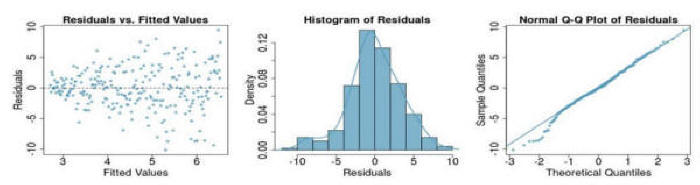
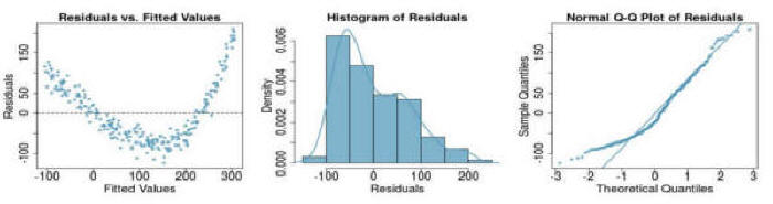
Question 3:  If you see the following residual versus fitted, distribution, and QQ plot after fitting a linear regression to the data, which of the following statements are true: (a) there is a linear upward trend, (b) there is a linear downward trend, (c) there is curved upward trend, (d) there is a curved downward trend, (e) there is a fanned shaped trend:

• Answer in More►

Question 4:&  If you see the following residual versus fitted, distribution, and QQ plot after fitting a linear regression to the data, which of the following statements are true: (a) there is a linear upward trend, (b) there is a linear downward trend, (c) there is curved upward trend, (d) there is a curved downward trend, (e) there is a fanned shaped trend:

• Answer in More►

More

For additional information (not part of the required reading), please see the following links:

1. Introduction to regression by others YouTube► Slides►
2. Regression using R Read►
3. Statistical learning with R Read►
4. Open introduction to statistics Read►

This page is part of the HAP 819 course on Advance Statistics and was organized by Farrokh Alemi PhD Home►  Email►