Supplement to Chapter on Comparison of Means

Presentations

1. Normal distribution  Slides►  Video►  YouTube►
2. Use Excel function for Z test YouTube►
3. Introduction to Control Chart  Slides► Listen►
4. X-bar chart lecture Slides► Listen►
5. XmR chart Slides► Listen►
6. Risk Adjusted X-bar chart lecture  Slides►  Listen►
7. Use Excel to create X-bar chart  Excel 2003► Video► SWF►
8. Use Excel to create risk adjusted X-bar chart  Excel 2003► 
9. Dot plots and the mean  Video►
10. Histograms and shape  How to►  How to►  Video►
11. Two sample Z test Video►
12. Calculating Z scores Video► Online Calculator►

Narrated slides and videos require Flash.

Assignments

Question 1.  In Health Administration Programs conducting satisfaction surveys are usually covered in courses on quality improvement.  This exercise shows how data from satisfaction surveys can be analyzed over time. Assume that, in different time periods, 4 randomly selected patients rated their satisfaction with our services.  Are we improving? Data► Answer►

Question 2.  In Health Administration programs accounting courses typically cover cost data.  Forensic accounting examines tries to detect fraud through accounting procedures. Following data were obtained regarding the cost of taking care of patients over several time periods.  Are our costs within expectation? Data► Slides► Listen► Answer►

Question 3: Payment reform has made hospital payments more complex.  One issue in payment reform is whether the net payments to hospitals is decreasing because of numerous carve outs for never-events.  In health administration program payment reform is covered in several courses including courses on value-based payments.  In this assignment, examine if payments for AMI to hospitals that received higher payment at start of 2015 has changed over time.  You can use Access database for opening the data in this assignment. You can analyze the data using Access SQL or Microsoft SQL.  Downloading these data files and linking them is a time consuming activity, allocate sufficient time to this activity. Keep the databases you download, we will repeatedly rely on the Hospital Compare data. Download dated data files from the archives. These files look like HosArchive_YYYYMMDD.zip, where YYYY is the year, and MM is the month. Unzip the files. Extract Hospital.mdb files for each time period, make sure you record the year and the month into the database name. Keep in mind that start and end periods of data are also given inside the files and that these do not correspond to the database year file.  Also note that the name of variables and files change over the years. Start from 1/1/2015 till the most recent available database. Since the data on AMI payments does not change in several of the files, you can save time and analyze the following 3 files:

In these files the denominator indicates the number of patients.  Payment indicates average payment per patient.  Select data that meet the following conditions:

1. Select the "PAYM_30_AMI" measure
2. Select hospitals who at start of 2015 had greater than national average payment.  This information is provided in the field [Compared to National] in the file [HQI_HOSP_AMI_Payment ]. 
3. Select hospitals that in the denominator do not have "Not Available".
4. Examine if the payments to the hospitals changed over time.  Create a control chart for the data.

Submit an Excel file containing the control chart for the data. Download►2016-11-10.zip► 2015-07-16.zip► 2015-01-22.zip►  Guide► Answer► Anto's SQL►

Question 4: Insurance companies and government payers are often interested in whether providers are billing their customary rate or whether they have increased their fees in contrast to the expected rate. In courses on forensic accounting, value-based payments, and quality, one often sees comparison of provider's current charges to expected charges. Using the data downloaded in question 3, create a risk-adjusted control chart for the last time period.  Use the average cost in the previous time period as expected value of payment for each hospital.  Compare the observed average payment to the expected (last time period's average) payment.  The steps you need to follow are the following:

1. For all hospitals (not just those that were above national average payment in 2015), create a table containing the most recent payment and the previous time period's  payment. 
2. Remove any hospital that did not have sufficient data in either time period.
3. Calculate if the recent payment is different from payment in the previous time period.
4. Test hypothesis that hospitals are receiving significantly higher payment at alpha levels less than 0.05.  You can use Excel's paired t-test to carryout this test.

Submit SQL code, top 5 organizations with highest and lowest increase in payment, and result of your test of the hypothesis. Download►2016-11-10.zip► 2015-07-16.zip► 2015-01-22.zip►

Question 5: Calculate the Probability of observing Z values in the following ranges in a normal distribution.  Answers are provided, show your intermediary table look-up values and calculations. Z calculator► Answer►

Question 6: Using the databases from Hospital Compare, download quarterly data on average number of hours of restraints from the file "HOSPITAL_QUARTERLY_QUALITYMEASURE_IPFQR_HOSPITAL".  Examine the data for "UNIVERSITY OF ALABAMA HOSPITAL".  This is hospital ID code 010023.  Not all time periods include new data.  I was able to find the following set of data (you can f ind more):

Numerator (Overall Hours of Restraint Use)	Denominator (Overall Number of Patients)	Start Date for Data Collection	End Date for Data Collection
3.15	4,449	10/1/2012	3/31/2013
18.18	9,226	4/1/2013	12/31/2013
59.06	12,878	1/1/2014	12/31/2014

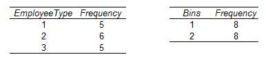
 Note that the field HBIPS-2_Overall_Num indicates the numerator for the measure "Hours of physical-restraint use."  The denominator for the same overall measure is in the field HBIPS-2_Overall_Den.  The dictionary provides the interpretation of these two fields as hours of restraint and number of patients examined. Using the procedure for XmR control chart examine if the total number of hours of restraints has changed over time. Download►2016-11-10.zip►2016-08-10.zip► 2016-05-04.zip► 2015-12-10.zip► 2015-10-08.zip► 2015-07-16.zip► 2015-05-06.zip► 2015-04-16.zip► 2015-01-22.zip►Dictionary►

Question 7: Find the value of standard normal variable z such that area under the curve below z is .3300 or .1003.  z Calculator►

Question 8: Variable X has a mean of 10 and standard deviation of 2 in the population. Calculate the z score that corresponds to X = 20. z Calculator►

Question 9: Variable X has a mean of 4 and standard deviation of 2 in the population. Find the value of X such that the corresponding z score for this value is -3. z Calculator►

Question 10: At a board meeting,  you hear different statements about who the clinic is serving.  According to the statements, 68% of the patients are under 25 years old and 10% are over 50 years old. Assuming that the patients are normally distributed, find the mean and standard deviation of the distribution.  We estimated the mean to be 10.62 and the standard deviation to be 30.74.  Show how these mean and standard deviations were calculated.  z Calculator►Answer►

Question 11: You are health administrator who is interested in examining organizational motivation and commitment of hospital employees. As part of a research project you have collected data from 16 employees serving in various wards of a hospital in a large metropolitan area. The following table provides information on Employee type (1 = trainee, 2 = supervisor, 3 = manager), Gender (1 = female, 2 = male), Training (0-10 scale), Motivation (0-10 scale), and Commitment (0-10 scale) of the 16 employees in your sample. Please make sure that you treat employees and gender as categorical variables and training, motivation and commitment as quantitative variables.

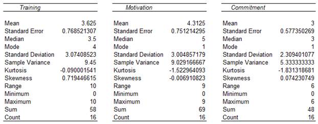
(a) Compute descriptive statistics for each variable.  Check that you have not made an error in data entry and that your descriptive statistics match the following Excel output.

(b) Use Excel to perform a one sample test to evaluate whether or not the mean motivation level of all employees in the population is different from 5. The null hypothesis is that µ1 = 5; i.e. the population mean motivation level is equal to 5. The alternative hypothesis is that µ1 ≠ 5; i.e. the population mean motivation level is significantly different from 5. Calculate the mean (4.31) and the standard deviation (3.00) using functions in Excel. Calculate the t-statistic and its degrees of freedom. Calculate the critical value and test if the critical value is less than alpha of 0.05. Copy/paste relevant Excel output. Provide interpretation of "t" test results.   

(c) Use Excel to perform a paired samples t-test to evaluate whether or not the mean Motivation level is significantly different from mean Commitment level in the population. The null hypothesis is that µ1 = µ2, i.e. the sample mean motivation level is equal to the sample mean commitment level. The alternative hypothesis is that  µ1 ≠  µ2, i.e. the sample mean motivation level is significantly different from the sample mean commitment level. Test at alpha levels less than 0.05. Copy/paste relevant Excel output. Provide interpretation of t-test results. Answer► 

(d) Use Excel to perform an independent samples t-test (assuming equal variances) to evaluate whether or not the mean Motivation level differs significantly between male and female employees in the population. The null hypothesis is that µ1 = µ2; i.e. the sample mean motivation level for females is equal to the sample mean motivational level for males. The alternative hypothesis is that µ1 ≠  µ2; i.e. the sample mean motivation level for females is significantly different from the sample mean motivational level for males. Copy/paste relevant Excel output. Provide interpretation of t-test results. For this problem you can assume that a pooled variance test is appropriate and alpha level is 0.05. Answer►

More

• Information on calculation of standard deviations Google►
• Annotated bibliography of using control charts to improve health care.  PubMed►
• Student-t distribution More►
• Badii's lecture on normal distributions Part 1► Part 2►Slides► SPSS tutorial►
• Measures of central tendency Video► SPSS tutorial►