George Mason University HAP 719 Advanced Statistics

HAP 719: Advanced Statistics I

Ordinary Regression Model Building  


Overview

Learning Objectives

After completing the activities this module you should be able to:

  • Examine if combination of variables are more accurate predictor than each variable by itself.
  • Distinguish among several methods of building a multiple linear regression model, including models with interaction terms
  • Interpret findings from statistical outputs pertaining to a regression model building technique

Coefficient of Determination

Coefficient of determination or R-squared is used to measure goodness of fit between the model and the data.  The statistic R2 measures the percentage of variation in the outcome (response variable in the regression) explained by the independent variables.  If a regression has a low R-squared then the right variables have not been included in the analysis, something often referred to as a model specification bias. In R, you can calculate the coefficient of determination (R-squared) for a linear regression model using the summary() function applied to the linear regression model object.  Here's how to calculate it. Assuming you have already fitted a linear regression model, which we'll call model, using a dataset called mydata, you can calculate R-squared as follows:

 # Fit the linear regression model
model <- lm(dependent_variable ~ independent_variable1 + independent_variable2, data = mydata)
# Calculate R-squared summary(model)$r.squared

In this code: lm() is used to fit the linear regression model, where dependent_variable is the variable you're trying to predict, and independent_variable1 and independent_variable2 are the independent variables in your model. summary(model) generates a summary of the regression model. $r.squared extracts the R-squared value from the summary.

After running this code, you'll get the R-squared value, which is a number between 0 and 1. A higher R-squared value indicates that a larger proportion of the variability in the dependent variable is explained by the independent variables, which suggests a better fit of the model to the data.

  • Read Chapter 11 in Statistical Analysis of Electronic Health Records, pages 277 to 280

Model Selection

To do regression, you have to try different mathematical models and see which one fits the data best.  A linear model is just a weighted sum of independent variables.  A non-linear model is a weighted sum of independent variables and interaction terms.  Interaction terms are constructed as product of 2 or more independent variable.   In R, you can run multiple regression models that take into account interactions among independent variables by including interaction terms in your regression formula. Interaction terms allow you to examine how the relationship between the dependent variable and one independent variable is influenced by another independent variable. Here's how to run such models. Let's assume you have a dataset named mydata and you want to run a multiple regression model that includes interactions between independent_variable1 and independent_variable2 along with other main effects:

# Fit a multiple regression model with interaction terms
model <- lm(dependent_variable ~ independent_variable1 * independent_variable2 + other_independent_variables, data = mydata)

In this example: dependent_variable is the variable you want to predict. independent_variable1 and independent_variable2 are the independent variables for which you want to test the interaction effect. other_independent_variables represents any other independent variables you want to include in the model as main effects. The * operator between independent_variable1 and independent_variable2 creates an interaction term. You can also explicitly define interaction terms using the : operator or the interaction() function:

# Using the : operator
model <- lm(dependent_variable ~ independent_variable1 + independent_variable2 + independent_variable1:independent_variable2 + other_independent_variables, data = mydata)
# Using the interaction() function
model <- lm(dependent_variable ~ independent_variable1 + independent_variable2 + interaction(independent_variable1, independent_variable2) + other_independent_variables, data = mydata)

 When you have a large number of variables (such as x1 through x15) and you want to include two-way interaction terms for all pairs of these variables in a linear regression model in R, it can be cumbersome to write out each interaction term manually. Fortunately, R provides functions to help automate the process. You can use the interaction() function in combination with the : operator. Here's how to calculate two-way interaction terms for all pairs of variables:

# Assuming you have a data frame called "mydata" with variables x1 through x15
# Create all possible two-way interactions
interaction_terms <- combn(names(mydata), 2, FUN = function(pair) interaction(mydata[[pair[1]]], mydata[[pair[2]]]), simplify = FALSE)
# Combine the interaction terms into a formula interaction_formula <- as.formula(paste("y ~", paste(interaction_terms, collapse = " + ")))
# Fit the regression model
model <- lm(interaction_formula, data = mydata)

In this code: combn() generates all possible combinations of variable pairs. The interaction() function is applied to each pair of variables to create interaction terms. as.formula() is used to convert the interaction terms into a formula. Finally, the linear regression model is fitted using the formula that includes all two-way interaction terms. Keep in mind that including a large number of interaction terms can lead to a more complex model and may require careful consideration of model selection and potential issues like multicollinearity. You may also want to assess the significance of the interaction terms and consider variable selection techniques if you have many variables and interactions.

After fitting the model, you can use summary(model) to obtain detailed information about the regression results, including coefficients, standard errors, p-values, and R-squared values. Interpreting the results of a multiple regression model with interaction terms involves considering the main effects of the independent variables and the interaction effects. For example, if independent_variable1 and independent_variable2 have a significant interaction effect, it means that the relationship between the dependent variable and independent_variable1 depends on the value of independent_variable2, and vice versa. Remember to assess the significance of interaction terms and their practical implications when interpreting the results. Additionally, be cautious about multicollinearity when including interaction terms, as it can affect the stability and interpretability of the coefficients. 

  • Read Chapter 11 in Statistical Analysis of Electronic Health Records page 274 to to 277
  • YouTube►

Assignments

Assignments should be submitted in Blackboard. The submission must have a summary statement, with one statement per question. All assignments should be done in R if possible.

Question 1: The following data provide a large number of factors that affect vaccination rates for COVID-19 in a county in United States.  Use hierarchical modeling to see which subset of factors explain largest portion of variance in getting Complete Series Vaccination rate.

Social-determinants,-political-leaning,-and-vaccination-hesitancy

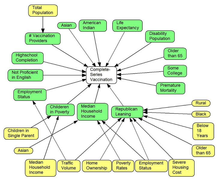
  1. Initially explain variation in Complete Series Vaccination rates by demographics (including age, race, gender) of the county's residents.  Report the percent of variation explained. 
  2. Explain variation in Complete Series Vaccination rates by demographics (age, race, gender), and social determinants (including high school completion rate, percent nor proficient in English, percent employed, percent of children in poverty, and median household income).  Report the percent of variation explained.
  3.  Explain variation in Complete Series Vaccination rates by demographics (age, race, gender), social determinants (including high school completion rate, percent nor proficient in English, percent employed, percent of children in poverty, median household income) and health of residents (including percent population disabled, life expectancy, percent population having premature morbidity).  Report the percent of variation explained.
  4. Explain variation in Complete Series Vaccination rates by demographics (age, race, gender), social determinants (including high school completion rate, percent nor proficient in English, percent employed, percent of children in poverty, median household income), health of residents (including percent population disabled, life expectancy, percent population having premature morbidity), and political leaning of the population (including republican leaning, democrat leaning).  Report the percent of variation explained.
  5. Does a county's political leaning affect vaccination rates?

Resources for Question 1:

Question 2: The following data provide a large number of factors that affect diabetes rate in a county in United States.  Use hierarchical modeling to see which subset of factors explain largest portion of variance in rate of diabetes in the county.

Network-model-of-diabetes-over-two-years.

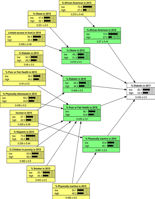
  1. Using only independent variables measured in 2015 predict incidence of diabetes in the county. Report the percent of variation explained.
  2. Using only independent variables measured in 2016 predict incidence of diabetes in the county. Report the percent of variation explained.
  3. Using both independent variables measured in 2015 and independent variables measured in 2016, predict incidence of diabetes in the ocunty. Report the percent of variation explained.
  4. List variables that have have an impact on incidence of diabetes within a year.
  5. List variables that have an impact on incidence of diabetes within 2 years.

Resources for Question 2:

More

For additional information (not part of the required reading), please see the following links:

  1. Introduction to regression by others YouTube► Slides►
  2. Regression using R Read►
  3. Statistical learning with R Read►
  4. Open introduction to statistics Read►

This page is part of the HAP 819 course on Advance Statistics and was organized by Farrokh Alemi PhD Home►  Email►