|
Generated by ChatGPT
Overview
In this module, you will explore linear ordinary regression, a
fundamental technique in statistical analysis. You will learn to transform
data to ensure that residuals have a Normal distribution, interpret the
output of ordinary regression, and test null hypotheses related to model
fit and variable relationships. With these skills, you will be able to
analyze data and uncover valuable insights, making you a valuable asset in
any data-driven field.
Learning Objectives
After completing the activities this module you should be able to:
- Analyze data using linear regression
- Transform data to have residuals that have a Normal distribution
- Interpret output of ordinary regression
- Test null hypothesis that a regression model has no fit with the
data
- Test null hypothesis that an independent variable is related to
the dependent variable
Lecture
 Indicates
AI assisted content, image or video. Indicates
AI assisted content, image or video.
Assignments
Assignments should be submitted in Blackboard. The submission must
have a summary statement, with one statement per question. All
assignments should be done in R if possible.
 Question 1: Clean the Medical Foster Home
data. Limit the data to cost per day, patient disabilities in 365
days, survival, age of patients, gender of patients and
whether they participated in the medical foster home (MFH) program.
Clean the data using the following: Question 1: Clean the Medical Foster Home
data. Limit the data to cost per day, patient disabilities in 365
days, survival, age of patients, gender of patients and
whether they participated in the medical foster home (MFH) program.
Clean the data using the following:
- Remove all cases in which all values for disabilities in 365
days, age and gender, are missing. These are meaningless
data and should be dropped from analysis.
- Remove any row in
which the treatment variable (MFH) is missing. MFH is an
intervention for nursing home patients. In this program, nursing home
patients are diverted to a community home and health care services are
delivered within the community home. The resident eats with the family
and relies on the family members for socialization, food and comfort.
It is called "foster" home because the family previously living in the
community home is supposed to act like the resident's family. Enrollment
in MFH is indicated by a variable MFH=1. A value of NaN or null is
missing value.
- Various costs are reported in the file,
including cost inside and outside the organization.
Rely on cost per day. Exclude patients who have 0 cost per day within the
organization. These do not make sense. The cost is reported for specific time period after
admission, some stay a short time, and others some longer. Use daily cost so you do not
get caught on the issues related to lack of follow-up.
- Select for your independent variables the probability of
disability in 365 days. These probabilities are predicted
from CCS variables. CCS in these data refer to Clinical
Classification System of Agency for Health Care Research and
Quality. CCS data indicate the comorbidities of the patient.
When null, it is assumed the patient did not have the comorbidity.
When data are entered it is assumed that the patient had the comorbidity
and the reported value is the first (maximum) or last (minimum) number of
days till admission to either the nursing home or the MFH. Thus an
entry of 20 under the minimum CCS indicates that from the most recent occurrence of the comorbidity
till admission was 20 days. An entry of 400 under the Maximum CCS indicates that from the
first time the comorbidity occurred till admission was 400 days. Because
of the relationship between disabilities and comorbidities, you
can rely exclusively on disabilities and ignore comorbidities.
- Check if cases repeat
and should be deleted from the analysis.
- Convert all categorical variables to binary dummy variables.
For example, race has four values W, B, A, Other, and null value.
Create 5 binary dummy variables for these categories and use 4 of
them in the regression. For example, the binary variable
called Black is 1 when race is B, and 0 otherwise. In this
binary variable we are comparing all Black residents to non-Black
residents that include W, A, null, and other races.
- In all variables where null value was not deleted row wise,
e.g. race being null, the null value should be made into a dummy
variable, zero when not null and 1 when null. Treat these
null variables as you would any other independent variable.
- Gender is indicated as "M"
and "F"; revise by replacing M with 1 and F with 0.
- Make sure
that no numbers are entered as text
- Visually check that cost is
normally distributed and see if log of cost is more normal than cost
itself. If a variable is not normally distributed, is the average of
the variable normal (see page 261 in required textbook)?
Visually check that age and cost have a linear relationship.
- Regress cost per day on age (continuous
variable), gender (male=1, Female=0), survival, binary dummy variables for race, probabilities of functional disabilities,
and any null dummy variable you have created.
- Show which variables have a
statistically significant effect on cost. Does age affect cost?
Does MFH reduce cost of care?
- Data
Download►
- Python's Teach Ones
- CCS codes Read►
- See sample R codes in required textbook pages 266 to 274 for doing the regression
- Vladimir Cardenas's Answer►
R-code►
- Aaron Jackson Hill's Teach One YouTube►
- Chethana Banoth's Teach One for R YouTube►
Question 2: Regress Circulatory Body System factor on all variables that precede it (defined as variables that occur more before than after
circulatory events). In the attached data, the variables indicate incidence of diabetes (a binary variable) and progression of diseases in body systems. You can do the analysis first on 10% sample before you do it on the entire data that may take several hours.
- Check the normal distribution assumption of the response variable.
Drop from analysis any place where the dependent variable is missing. If the data is not normal; transform the data to meet normal assumptions.
For each transformation show the test of Normal distribution. You
should at a minimum consider the following transformations of the
data:
- Odds to probability transformation
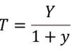
- Log of odds to probability transformation
- Logarithm transformation:
- Third root of odds

- Check the assumption of linearity. If the data have non-linear elements, transform the data to remove non-linearity.
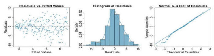
Question 3: If you see the following residual versus fitted, distribution, and QQ plot after fitting a linear regression to the data,
which of the following statements are true: (a) there is a linear upward trend, (b) there is a linear downward trend, (c) there is curved upward
trend, (d) there is a curved downward trend, (e) there is a fanned shaped trend:
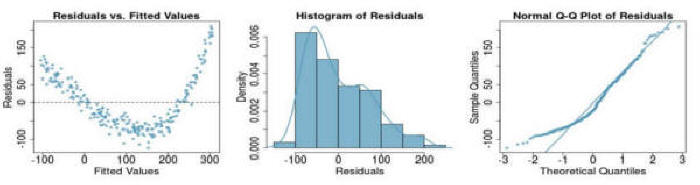
Question 4: If you see the following residual versus fitted, distribution, and QQ plot after fitting a linear regression to the data,
which of the following statements are true: (a) there is a linear upward trend, (b) there is a linear downward trend, (c) there is curved upward
trend, (d) there is a curved downward trend, (e) there is a fanned shaped trend:
Question 5: The attached data comes from Larry Hatcher's book
titled "Advanced Statistics in Research" The response variable is
average of grades in graduate school and the independent variables are
listed in the following table are admission information:
If your instructor has not covered this topic, please learn from
ChatGPT. Please answer the following questions:
- What does adjusted R2 measure and "according to the criteria
recommended by Cohen (1988), does this value of R2 come closest to
representing a zero effect, a small effect, a medium effect, or a
large effect?"
- "According to Table E9.3.2, the unstandardized multiple regression
coefficient for undergraduate GPA overall is b = 0.313. What does this
value mean? In other words, what is the correct interpretation of this
coefficient (hint: your answer must incorporate the definition for an
unstandardized multiple regression coefficient, and it must also
incorporate the value “0.313”)."
- Which variables have a statistically significant relationship with
graduate grades?
- "What was the unstandardized multiple regression coefficient
for undergraduate GPA overall?"
- "What was the 95% confidence interval for this coefficient?"
- "Assume that you had access to this 95% confidence interval but
not the p value for the regression coefficient. Based only on this 95%
confidence interval, was this regression coefficient statistically
significant? How do you know?"
- Is the statistical test of the coefficient for undergraduate GPA's
affected by other variables in the model? How is the test of
coefficient in a regression model different from hypothesis testing of
the same variable by itself and without other variables in the
regression model. Explain your answer.
- "If an applicant increased his or her GRE quantitative test score
by one standard deviation, that applicant’s score on graduate GPA
overall would be expected to increase by how many standard deviations
(while statistically controlling the remaining predictor variables)?"
- "What percent of variance in graduate GPA overall is accounted for
by the GRE verbal test, above and beyond the variance already
accounted for by all of the other predictors?"
- Is the GRE verbal test more useful in predicting graduate grades
than the GRE quantitative test?
- Does the model capture interaction among the variables?
More
For additional information (not part of the required reading), please see the following links:
- Introduction to regression by others
YouTube►
Slides►
- Regression using R Read►
- Statistical learning with R
Read►
- Open introduction to statistics
Read►
This page is part of the HAP 819 course on Advance Statistics and was
organized by Farrokh Alemi PhD Home►
Email►
|